


Table of Contents
Trying to learn too fast and skipping essential knowledge is a mistake many new machine learning practitioners make. It’s easy to underestimate the importance of proper model evaluation. Choosing the right way to evaluate a classification model is as important as choosing the classification model itself, if not more. Sometimes, accuracy might not be the best way to evaluate how a classification model performs.
For real-world applications, a bad model evaluated as a high-quality model is very dangerous and can lead to serious repercussions. You need to know that a model underperformed in order to improve it.
In this article, I am going to explain the different methods used for evaluating results from classification models. Knowing when to use each method comes with experience, but learning about each of these methods is a great place to start.
What is Classification Accuracy?
Accuracy is the conventional method of evaluating classification models. Accuracy is defined as the proportion of correctly classified examples over the whole set of examples.
Accuracy = (Number of correct predictions) / (Overall number of predictions)
Accuracy is very easy to interpret, which is why novices tend to favor it over other methods. In practice, it is only used when the dataset permits it. It is not completely unreliable as a method of evaluation, but there are other, and sometimes better, methods that are often overlooked.
When you only use accuracy to evaluate a model, you usually run into problems. One of which is evaluating models on imbalanced datasets.
Let's say you need to predict if someone is a positive, optimistic individual or a negative, pessimistic individual. If 90% of the samples in your dataset belong to the positive group, and only 10% belong to the negative group, accuracy will be a very unreliable metric. A model that predicts that someone is positive 100% of the time will have an accuracy of 90%. This model will have a "very high" accuracy while simultaneously being useless on previously unseen data.
Because of its shortcomings, accuracy is often used in conjunction with other methods. One way to check whether you can use accuracy as a metric is to construct a confusion matrix.
How to Construct a Confusion Matrix
A confusion matrix is an error matrix. It is presented as a table in which the predicted class is compared with the actual class. Understanding confusion matrices is of paramount importance for understanding classification metrics, such as recall and precision. The rows of a confusion matrix represent real values, while the columns represent predicted values. I'll demonstrate how a confusion matrix would look for the previous example of classifying people into positive and negative individuals.
Confusion Matrix
| Predicted Value | |||
| Positive | Negative | ||
| Real Value |
Positive | TP | FP |
| Negative | FN | TN | |
Reading a confusion matrix is relatively simple:
True Positive (TP): you predicted positive, the real value was positive
True Negative (TN): you predicted negative, the real value was negative
False Positive (FP): you predicted positive, the real value was negative
False Negative (FN): you predicted negative, the real value was positive
Using the values inside the confusion matrix, you can calculate the metrics that you use for the purposes of evaluating classification models.
Those metrics are:
- Precision (also known as Positive Predicted Value)
- Recall (also known as Sensitivity or True Positive Rate)
- Specificity (also known as Selectivity or True Negative Rate)
- Fall-out (or False Positive Rate)
- Miss Rate (or False Negative Rate)
- Receiver-Operator Curve (ROC Curve) and Area Under the Curve (AUC)
Precision (Positive Predicted Value)
Precision is defined as the number of true positives divided by the sum of true and false positives. Precision expresses the proportion of data correctly predicted as positive. Using it as a metric, you can define the percent of the predicted class inside the data you classified as that class. In other words, precision helps you measure how often you correctly predicted that a data point belongs to the class your model assigned it to. The equation for it is:
Precision = (True Positive) / (True Positive + False Positive)
Recall (Sensitivity, True Positive Rate)
The recall is defined as the number of true positives divided by the sum of true positives and false negatives. It expresses the ability to find all relevant instances in a dataset. Recall measures how good your model is at correctly predicting positive cases. It’s the proportion of actual positive cases which were correctly identified. The equation for recall is:
Recall = (True Positive) / (True Positive + False Negative)
Article continues below
Want to learn more? Check out some of our courses:
Precision/Recall Tradeoff
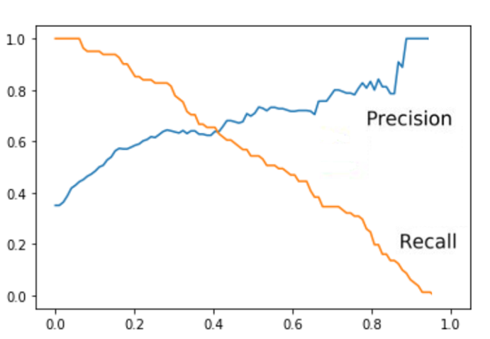
In an ideal scenario, where your data is perfectly separable, you could achieve a value of 1.0 for both precision and recall. In most practical situations, that is impossible, and a tradeoff arises: increasing one of these two parameters will decrease the other. By virtue of that tradeoff, you should seek to define what we call an optimal threshold. An optimal threshold will lead to an optimal tradeoff. This threshold doesn't necessarily achieve a perfect balance between precision and recall. The situation at hand might need a tradeoff that is biased towards one of them.
This will vary from situation to situation. A typical example is high-risk scenarios, such as classifying patients by whether they are at risk of having a heart attack or not. In these situations, being biased towards recall is preferable. It is more important that you classify all patients that can potentially have a heart attack as positive, even if you get a few extra false positives in that class. Having very high precision in such a case is a luxury. You should aim for high recall, even if you somewhat sacrifice precision. Although I sometimes take a biased tradeoff, most of the time I prefer a good balance between precision and recall. The easiest way to find that balance is to look at a graph that contains both the precision and the recall curves.
Image Source: Precision and Recall tradeoff, Edlitera
Optimizing the precision/recall tradeoff comes down to finding an optimal threshold by looking at the precision and recall curves. The easiest way to be sure that you set your balance right is the F1 Score.
F1 Score
The F1 score is easily one of the most reliable ways to score how well a classification model performs. It is the weighted average of precision and recall, as defined by the equation below.
F1 = 2 [(Recall * Precision) / (Recall + Precision)]
You can also transform the equation above to a form that allows you to calculate the F1 score directly from the confusion matrix:
F1 = (True Positive) / [True Positive + 1/2*(False Positive + False Negative)]
The F1 score makes sure that you achieve a good balance between precision and recall. Whenever any of those two values is low, the F1 score will also be low. A high F1 score is a good indicator that your model performs well, since it achieves high values for both precision and recall.
Specificity (Selectivity, True Negative Rate)
Specificity is similar to sensitivity, only the focus is on the negative class. It is the proportion of true negative cases which were correctly identified as such. The equation for specificity is:
Specificity = (True Negative) / (True Negative + False Positive)
Fall-out (False Positive Rate)
Fall-out determines the probability of determining a positive value when there is no positive value. It is the proportion of actual negative cases that were incorrectly classified as positive. The equation for fall-out is:
Fall-out = (False Positive) / (True Negative + False Positive)
Miss Rate (False Negative Rate)
Miss rate can be defined as the proportion of positive values that were incorrectly classified as negative examples.
Miss Rate = (False negative) / (True positive + False negative)
Receiver-Operator Curve (ROC Curve) and Area Under the Curve (AUC)
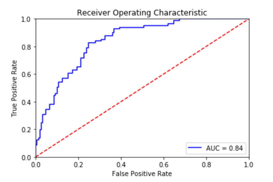
Receiver-operator curve, or ROC, curves display the relationship between sensitivity and fall-out. They work by combining the confusion matrices at all threshold values. The result is a summary of the model’s performance, displayed in the form of a curve.
This curve allows you to find a good probability threshold. Probability thresholds are decision points used by the model for classification. They define the minimum predicted positive class probability resulting in a positive class prediction.
Image Source: ROC curve and AUC score, https://towardsdatascience.com/roc-curve-in-machine-learning-fea29b14d133
The best model is the one with a curve away from the dashed line. The dashed line represents a 50% chance of guessing correctly, so the further away you are from it, the better. To decide which model performs best, you can also look at the area under the curve, or AUC, value. AUC size is directly connected to model performance. Models that perform better will have higher AUC values. A random model will have an AUC of 0.5, while a perfect classifier would have an AUC of 1.
What Are Special Cases for Classification Models?
There are some special cases. You are mostly talking about losses that are predominantly used with neural networks. Neural networks function differently than standard machine learning algorithms. The two basic metrics used to define how well a neural network model performs are:
- Binary Cross-Entropy
- Categorical Cross-Entropy
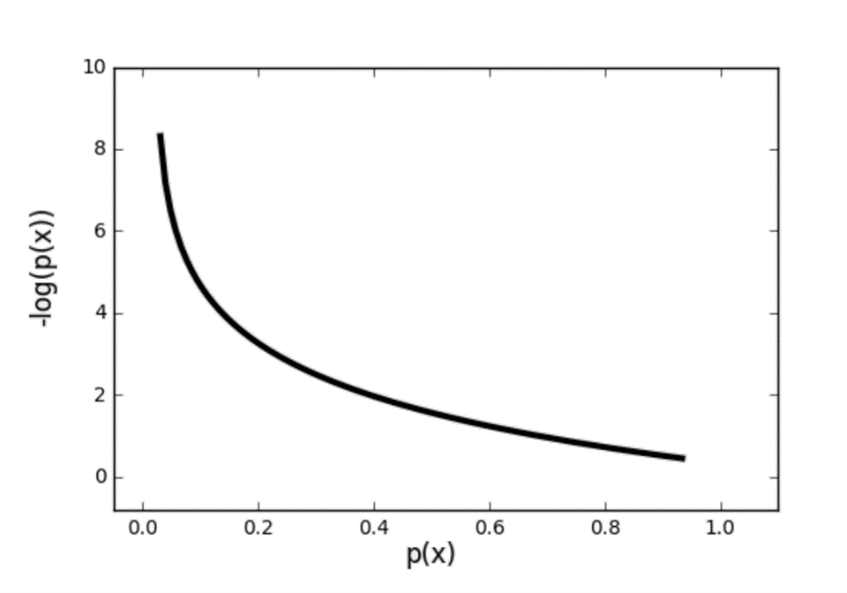
Binary Cross-Entropy
Binary cross-entropy is used when dealing with binary classification problems. Binary cross-entropy is also known as log loss. As a metric, it is mainly used in neural networks. Binary cross-entropy considers the uncertainty that comes with predictions. It considers how much a prediction varies from the actual label. This leads to increased performance and better results, but it also leaves the model susceptible to problems that arise from imbalanced datasets. When dealing with imbalanced datasets, you need to modify binary cross-entropy. Class weight or some other type of constraint needs to be introduced to make sure that the metric accurately evaluates the quality of your model.
Image Source: Binary Cross-Entropy, https://towardsdatascience.com/understanding-binary-cross-entropy-log-loss-a-visual-explanation-a3ac6025181a
Categorical Cross-Entropy
Categorical cross-entropy is used when dealing with multiclass problems. Binary cross-entropy generalizes well for multiclass problems. That generalization is what we call categorical cross-entropy. Therefore, categorical cross-entropy brings about both the same benefits and problems that go along with using binary cross-entropy.
A Classification Model Evaluation Example
As a demonstration, I am going to train a logistic regression model and evaluate it using some of the methods from this article. I will use the "pima-indians-diabetes-classification" dataset that is used for demonstrations.
- Defining Data Science Experiments and How to Set Up a Successful One
- Data Science Success: Knowing When and How to Make Decisions Based on Data Science Results
The demonstration will be separated into four steps:
- Loading the necessary modules
- Loading and preparing the data
- Defining and training the model
- Evaluating the model
Each of these steps will be explained. The code for each step will also be provided.
First Step: Load the Necessary Modules
The first step is simple, you just need to import the modules that will be used.
# Imports for loading in data

 import pandas as pd

 # Imports required for plotting

 import matplotlib.pyplot as plt
 %matplotlib inline

 # Imports required for transformations, splitting data and for the model

 from sklearn.preprocessing import MinMaxScaler
 from sklearn.model_selection import train_test_split
 from sklearn.linear_model import LogisticRegression


 # Imports required for model evaluation

 from sklearn.metrics import roc_auc_score
 from sklearn.metrics import roc_curve,auc
 from sklearn.metrics import confusion_matrix, classification_report, accuracy_score
Second Step: Load and Prepare the Data
In this step, you need to load in your data, shuffle it, prepare datasets, and scale your data. After loading the data, you’ll need to shuffle it to make sure that it isn't sorted in any way before you separate it into train and test datasets. After separating the data into datasets, you need to scale it. This way you make sure that different magnitudes of data won't influence your model’s performance.
 # Load in data

 data = pd.read_csv("pima-indians-diabetes-classification.csv",
                    names = ["pregnancies", "clucose", "blood_pressure",
                             "skin_thickness", "insulin", "bmi",
                             "diabetes_pedigree", "extra", "result"], header = None)

 # Data shuffle

 data = data.sample(frac=1).reset_index(drop=True)


 # Prepare data

 X = data.iloc[:,:-1]
 y = data.iloc[:,-1]

 X_train,X_test,y_train,y_test = train_test_split(X,y,stratify = y,test_size= 0.3,random_state=42)

 # Scale data

 scaler = MinMaxScaler()

 X_train = scaler.fit_transform(X_train)
 X_test = scaler.transform(X_test)
Third Step: Define and Train the Model
In the third step, you define your model and train it. In practice, you should always use more than one model, but since I am just showing a few different ways of evaluating the performance of a classification model, you will train just one logistic regression model.
# Prepare the model

 log_reg = LogisticRegression(solver="lbfgs")

 # Fit the model
 log_reg.fit(X_train, y_train)

 # Predict the target vectors
 y_pred_log_reg = log_reg.predict(X_test)
Note: The solver for the logistic regression model is strictly defined as "lbfgs" to make sure that the Sci-kit library will use the newest solver.
Fourth Step: Evaluate the Model
The fourth and final step is the most important one for this demonstration. Let's see how the model performed. To start with, you will check the accuracy score of the model. To do this, you can use the following code.
 #Print accuracy

 log_reg_accuracy = accuracy_score(y_pred_log_reg, y_test)
 print(f"Logistic regression accuracy: {round(log_reg_accuracy * 100)}%")
The resulting accuracy from the model is:
Logistic regression accuracy: 80.0%
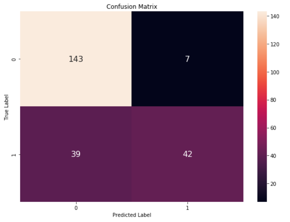
An accuracy score of 80% is really good for a logistic regression model in this case. But as I said before, accuracy is not the best metric for evaluating how a model performs. Following what I talked about in the article, let's construct a confusion matrix.
# Plot out a confusion matrix

 def plot_confusion_matrix(y_test, y_predicted):
     conf_mat = pd.DataFrame(confusion_matrix(y_test, y_predicted))
     fig = plt.figure(figsize=(10, 7))
     sns.heatmap(conf_mat, annot=True, annot_kws={"size": 16}, fmt="g")
     plt.title("Confusion Matrix")
     plt.xlabel("Predicted Label")
     plt.ylabel("True Label")
     plt.show()

 plot_confusion_matrix(y_test, y_pred_log_reg)
The resulting plot from that will show how the model really performs.
Image Source: The confusion matrix of the model, Edlitera
You could use the equations I defined earlier to calculate the F1 score, the precision, and other metrics, but sklearn allows you to print out a "classification report" using a minimal amount of code.
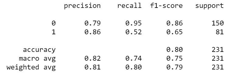
 # Print the precision, recall and f1-scores

 print(classification_report(y_test, y_pred_log_reg))
Let's see the result after running the code.
This classification report gives you a lot of information. You get the precision, recall, F1 score, and accuracy. You can see that your precision for both classes is relatively close, but you also see an enormous difference in terms of recall for the two classes. The difference between F1 scores is also sizable. This means the model didn't really perform as well as initially thought. You can further confirm this by plotting an ROC curve and calculating the AUC score.
 # Plot ROC curve and calculate AUC score

 def plot_roc_curve(X_test, y_test, model, model_name="Classifier"):
     # The line below is equivalent to
     # y_predicted = model.predict(X_test)
     y_predicted = getattr(model, "predict")(X_test)

     # The line below is equivalent to
     # y_predicted_proba = model.predict_proba(X_test)
     y_predicted_proba = getattr(model, "predict_proba")(X_test)

     auc_roc_log_reg = roc_auc_score(y_test, y_predicted)
     fpr, tpr, thresholds = roc_curve(y_test, y_predicted_proba[:,1])

     plt.plot(fpr, tpr, color="red", lw=2,
              label=f"{model_name} (area = {auc_roc_log_reg:0.5f})")
     plt.plot([0, 1], [0, 1], color="black", lw=2, linestyle="--",
              label="Mean model (area = 0.500)")
     plt.xlim([0.0, 1.0])
     plt.ylim([0.0, 1.05])
     plt.xlabel("False Positive Rate")
     plt.ylabel("True Positive Rate")
     plt.title("Receiver operating characteristic")
     plt.legend(loc="lower right")
     plt.show()

     # Calculate the auc score
     auc_score = auc(fpr, tpr)
     print(f"auc_score: {round(auc_score, 3)}.")

 plot_roc_curve(X_test, y_test, log_reg, "Logistic regression")
The resulting ROC curve, along with the AUC score looks like this:
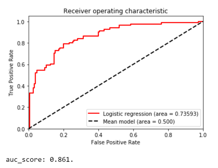
The ROC curve, along with the AUC score, confirms the previous assumptions. Even though the accuracy rate is a pretty good 80% and the ROC curve and AUC score support the success of this model, the difference in the recall rates and the F1 scores are worth investigating. In a real world use case, by testing out a few more models, you might be able to find a model, or models, that work better for your data. Besides, as I mentioned earlier, training more than one model is always recommended when it comes to machine learning.
Although it might seem like the obvious measurement for success, accuracy alone does not tell you all you need to know about a model’s performance. There are other methods and metrics that you can use alongside accuracy to ensure that your classification model meets your expectations. Join our Classic Machine Learning with Python courses to learn more!

