


Table of Contents
Previous article in series: Python Data Processing: How To Select Data in NumPy
This article is the last one in the series of articles on NumPy. In the previous articles, we talked about what NumPy is, what an ndarray is, how we manipulate data stored in them, and so on. All of those articles served as an introduction to this article, which covers how to perform various mathematical operations with NumPy, how to calculate statistics, and also how to transform ndarrays.
In this article, I'll cover the previous topics in as much detail as I can fit inside this limited format. Take note that NumPy, similar to other packages in Python, is too large to cover in just a small series of articles, but this final article will nicely wrap up all of the topics mentioned in the previous articles and can be used as a strong foundation for learning more about NumPy or moving on and learning about Pandas and other data processing and visualization libraries.
How to Perform Simple Operations
Before we dive deep into the intricacies of performing vectorized operations with NumPy, let's first go over some simpler operations. It is nonsensical to talk about stuff such as calculating the standard deviation of the elements inside an array before we cover the basics such as how to add a single element to an array, how to add a list to an array, and how to add one array to another, etc.
To add elements to an array, you use the append() function from NumPy. This function takes in a maximum of three arguments, where the first two are mandatory and the third argument is optional. The first argument you input is the original array, to which you want to add some element(s). The second argument is the element(s) you want to add to the original array. The third optional argument defines the axis you want to use when adding elements.
Let's demonstrate how the function works on a simple example: I will create an array called nums and add the integer 6 to it. We will store the new array with the added element into a new array called nums_2.
# Create the original array
nums = np.array([1, 2, 3, 4, 5])

# Add the integer 6 to the original array
# and store the result in a new array
nums_2 = np.append(nums, 6)
The result of the previous operations, the array nums_2, will be a one-dimensional ndarray that will contain the integers 1, 2, 3, 4, 5, and 6. So as you can see, adding a single element is pretty easy.
Adding a list to a one-dimensional array is achieved using pretty much the same syntax:
# Create the original array
nums = np.array([1, 2, 3, 4, 5])

# Add the integer 6 to the original array
# and store the result in a new array
nums_2 = np.append(nums, [6, 7, 8, 9, 10])
Once you start working with arrays that have more than one dimension, things start to get a bit tricky.
At this point, I'm basically talking about appending arrays to arrays. The fact that I'm appending one array to another one means that I must be very careful about the dimensions of the two arrays. The arrays need to have the same dimensions for the operations to work properly. Not only that, there is actually one additional thing to keep in mind. The default behavior of NumPy, when we try to add one array to another using append(), is to flatten the two arrays and create a one-dimensional array as a result. Therefore when adding one array to another, it is also a good idea to specify the axis to which we want to append the values to make sure the final array has the form we want it to have.
Let's demonstrate how this works with an example. I will create two two-dimensional arrays, arr_1 and arr_2, and will then demonstrate what the result would look like if we were to append them first on axis 0 and later on to axis 1.
# Create first array
arr_1= np.array([[1, 2], [3, 4]])

# Create second array
arr_2 = np.array([[5, 6], [7, 8]])

# Append arr_2 to arr_1
# on axis 0
np.append(arr_1, arr_2, axis=0)
# Append arr_2 to arr_1
# on axis 1
np.append(arr_1, arr_2, axis=1)
Now that I've explained how to add values to arrays, you are ready to move on to more complex operations.
Article continues below
Want to learn more? Check out some of our courses:
How to Perform Vectorized Operations
Now is the time to demonstrate the full power of NumPy: the efficiency with which NumPy performs vectorized operations. First, I'll explain how to perform various mathematical operations using NumPy, and later on, I'll demonstrate how you can use NumPy to calculate various statistics that help you better describe data stored in our arrays.
Of course, I won't cover every operation that exists since NumPy is a very extensive library. No article would be big enough to cover absolutely everything. I'll demonstrate on multiple examples how easy it is to perform complex operations using the API provided by NumPy. With just a line or two of code, you'll be able to solve any problem you run into.
How to Perform Math Operations With NumPy
Before moving on to basic statistics, let's demonstrate how we can perform mathematical operations using NumPy. This is probably going to be very familiar to those of you that remember a little bit of algebra, but even if you don't, you do not need to worry about it. NumPy does all the heavy lifting for us, making sure that all of the calculations give the correct results.
For example, if I try to multiply a one-dimensional array that consists of integers 1, 2, 3, and 4 with a scalar, let's say the integer 10, that operation will be applied element-wise. That means that each number inside my array will be multiplied by the scalar value, so my final result will be an array that consists of the integers 10, 20, 30, and 40.
# Create the example array
nums = np.array([1, 2, 3, 4])

# Multiply the elements in the array element-wise
nums * 10
The same rules apply if we, instead of multiplication, perform addition. The final result will be an array with the values 11, 12, 13, and 14 inside of it.
# Create the example array
nums = np.array([1, 2, 3, 4])

# Add 10 to the elements in the array element-wise
nums + 10
This shows how easy it is to perform these operations, but the real beauty of NumPy is in how it performs these operations. To be more specific, NumPy won't use loops to perform these calculations but will instead use a process called vectorization. Because NumPy knows for a fact that the data stored in the array is homogenous, it can delegate complex mathematical operations to optimized compiled code, which in turn leads to a tremendous speedup in comparison to how Python usually performs such operations.
The same will happen if we decide to work with two arrays instead of an array and a scalar. So if I multiply one array with another array, the elements inside those arrays are going to be multiplied element-wise. Just keep in mind that the two arrays need to match in size because you are performing the operation element-wise.
# Create first example array
nums_1 = np.array([1, 2, 3, 4])

# Create second example array
nums_2 = np.array([5, 6, 7, 8])
# Multiply the two arrays
nums_1 * nums_2
Of course, you can do much more than just addition, subtraction, multiplication, etc. NumPy has a lot of built-in operations that you can use to modify values inside arrays.
For example, the sqrt() function from NumPy will return an array of square roots of the numbers that were in the original array.
# Create the example array
nums = np.array([1, 2, 3, 4])

# Create an array of square roots
nums_sqrt = np.sqrt(nums)
All of the aforementioned barely scratches the surface. The number of in-built operations in NumPy is gigantic, and as previously mentioned all of them run on optimized compiled code so executing these operations takes very little time, even when you are working with extremely big arrays.
Now that I explained how performing mathematical operations works in NumPy, let's explain the basics of calculating some statistical values.
How to Perform Statistical Operations
The most important thing you need to keep in mind when we are talking about performing statistical operations is the previously explained concept of axes. Remember, when talking about arrays, we prefer using the terms axis 0 and axis 1 over the terms rows and columns. The reason for that is very simple. Even though there are situations where you want to operate on the whole array, such as to calculate the mean of all the values in the array, much more often you need to calculate the mean of each row or the mean of each column. In those cases, the concept of axes proves to be invaluable.
Let's demonstrate this with an example. If I want to calculate the mean of all the numbers in an array, I can just use the built-in mean() method from NumPy.
# Create the example array
nums = np.array([[1, 2, 3, 4], [5, 6, 7, 8]])

# Calculate the mean
# of all the numbers in the array
nums.mean()
While this can be useful information, you will typically be interested in calculating the mean (or other statistical measures) of columns or rows. This is where the concept of axes comes into play. To find information about rows, you look at axis 0 and, to find information about columns, you look at axis 1.
# Create the example array
nums = np.array([[1, 2, 3, 4], [5, 6, 7, 8]])

# Calculate the means
# of rows
nums.mean(axis=0)

# Calculate the means
# of columns
nums.mean(axis=1)
Of course, the mean() method is not the only method you can use. You can calculate the sum using the sum() method, the standard deviation using the std() method, the index of the minimum element using the argmin() method, etc.
Whatever you want to calculate, NumPy probably has a built-in method that will allow you to calculate that with a single line of code (as long as you are careful about applying the method on the right axis).
How to Use Conditional Logic to Transform Arrays
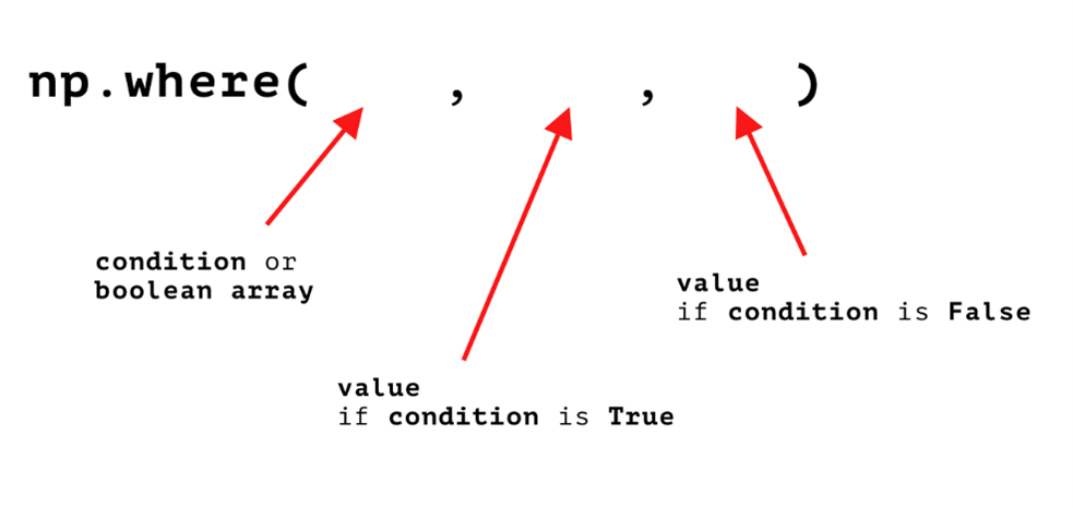
You can also transform arrays by applying conditional logic to them. To be more precise, you don't actually transform the original array, but you get a new version that you can then store in a new variable. The way you do this is pretty simple: you use the where() function from NumPy.
This function takes in three arguments, and is best described using the following visual aid:
Image Source: Three functional arguments for the where() method, Edlitera
The condition you enter, or the boolean array, is something you already talked about in a previous article (the one on boolean arrays, boolean indexing, and filtering). This condition is the same thing. Using it, you can tell NumPy to take a look at some array and return a copy of it with transformed values.
The second argument is typically what you want to transform the values of the original array to if they satisfy the previously given condition, while the third argument is the value that you want the transformed array to contain when the condition is not satisfied. Let's demonstrate it with an example.
First, let's create an example array:
# Create example array
arr = np.array([[0.64410602, -1.19373699],
            [-0.29749826,  1.58836562],
            [1.97135724,  0.63080637],
            [1.10235055,  0.317552]])
Now we can use the where() function from NumPy to transform it. You want the transformed array to contain 1 whenever the value in the original array was positive, and -1 whenever the value in the original array was negative. To do that, you are going to create a filter that checks that condition, input it as the first argument and then you are going to input 1 and -1 as the second and third arguments.
# Create transformed array
transformed_arr = np.where(arr > 0, 1, -1)
As you can see, the final array you end up with has the same shape as the original array, but it only contains the numbers 1 and -1. One very common thing that programmers do is they decide to transform only one value.
For example, instead of changing all negative values to -1, leave them as they are. To do that, just enter the original array name as the second argument and that will make sure that the values that don't satisfy the condition don't get changed.
# Create transformed array
transformed_arr = np.where(arr > 0, 1, arr)
transformed_arr
The where() function is very powerful, so you can even do very advanced stuff, such as enter mathematical formulas as the second and third argument, apply built-in functions, etc.
# Create example array
arr = np.array([[1, 2],
            [3, 4],
            [5, 6],
            [7, 8]])

# Create transformed array
transformed_arr = np.where(arr > 0, np.sqrt(arr), arr * 2)
The where() function allows you to do some pretty powerful stuff, and it is also extremely efficient. Even when you start using Pandas, there are some situations where using the where() function from NumPy will be preferable over using a built-in Pandas function because of how efficient it is.
This article demonstrated the real power of NumPy, which lies in its ease of use and efficiency. In it I explained using multiple examples and various concepts that bring together everything previously mentioned in this series of articles. The series itself serves as a great base for diving deeper into NumPy, but the main idea is that it explains the basic concepts that are used by higher-level libraries, such as Pandas, that use NumPy in the background.

