


Filtering data is an essential process and something that you will use frequently. It allows you to extract specific portions of your dataset that you consider relevant for your data analysis. Often, not all of the data that you have at your disposal is relevant to the analysis you want to perform. This article will cover how you can filter the data present in your DataFrame to access only those portions of it that are important for the task in progress.
Why Filter Data?
In the context of data processing and analysis, filtering is the process of selecting a subset of your total data based on certain specific criteria. Defining certain conditions allows us to separate a subset of our data that satisfies those criteria. Afterward, we can discard the remaining data that does not meet the conditions. There are many benefits to this.
First, filtering is one of the main data cleaning processes we perform. Therefore, this makes it an essential part of every data preprocessing pipeline. Cleaning data is essential when you want to perform a high-quality analysis of it but not only that. It is also instrumental in preparing it for different Machine Learning models or any other algorithms you plan on using in the future.
Second, we usually decrease the size of our dataset significantly with the help of filtering. This results in improving the performance of our data processing. Smaller datasets require less memory and computational power. This leads to a significantly faster execution of data operations.
Third, it is particularly easier to visually analyze data after filtering. Let us imagine working with a smaller subset of values that all share certain characteristics. This makes the creation of focused and interpretable charts and graphs a far easier process.
Article continues below
Want to learn more? Check out some of our courses:
How Do We Filter Data in Pandas
In Pandas, there are various methods to filter data, normally involving:
- filtering based on a single condition
- filtering based on multiple conditions
- filtering using a custom function
Let's demonstrate by filtering some example data stored in a Pandas DataFrame. For starters, I will create the example DataFrame so that there is data for manipulation:
import pandas as pd

# Create some example data
data = {
    "Name": ["Alice Smith", "Dave Johnson", "John Smith", "Diana Stockton", "Emily Brown", "Frank Castle", "Gina Davis", "John Potter", "Helen Davis"],
    "Age": [35, 25, 29, 37, 29, 53, 42, 31, 38],
    "Salary": [90000, 20000, 120000, 60000, 35000, 80000, 50000, 55000, 110000],
    "Department": ["Sales", "Janitorial Services", "IT", "HR", "Marketing", "Legal", "Operations", "Finance", "IT"],
    "HighEarner": ["Yes", "No", "Yes", "No", "No", "Yes", "No", "No", "Yes"]
}

# Create a DataFrame from the example data
df = pd.DataFrame(data)
The code above will create the following DataFrame and store it inside the df variable:
Now that we have this DataFrame at our disposal, let's demonstrate how we can filter the data in it in different ways.
How Do We Filter Data Based on a Single Condition
Filtering based on a single condition is the simplest type of filtering. This type of operation is quite similar to grouping, as it will essentially return a subset of data back that matches one single condition. The general syntax formula for filtering is really simple, and it relies on the usage of square brackets:
filtered_df = df[condition]
In the formula above, df represents the original DataFrame, condition is some Boolean expression that is used as criteria for filtering. The final result we get is the filtered_df DataFrame. In Pandas, the condition used for filtering must be a Boolean expression. This is because the filtering process is based on Boolean indexing. In such case, each row of the DataFrame is evaluated against a condition that returns either True or False.
To put it simply, including a Boolean expression inside square brackets in Pandas, will lead to row-wise evaluation. The result will be filtering the DataFrame to include only the rows that meet the specified condition. Therefore, what you finally get is a Boolean Series, a series of True and False values, that matches the length of the DataFrame. This Series then determines which rows are selected (those corresponding to True) and which are excluded (those corresponding to False) from the filtered version of our DataFrame.
For example, let's separate those that are older than 40:
# Filter based on age
condition = df['Age'] > 40
older_than_40 = df[condition]
The code above will store the following DataFrame in the older_than_40 variable:
What happens in the background when we run the code above is quite simple. The code will inform Pandas to keep only those rows from the original DataFrame where the condition df['Age'] > 40 evaluates to True. The rest will be discarded.
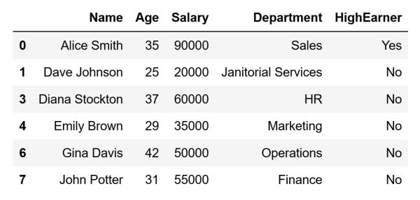
The condition used for filtering can certainly be whatever we want, as long as it is a Boolean expression. For instance, I can use filtering to select only those rows where the value in the HighEarner column is "Yes" by running the following code:
# Select high earners
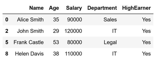
condition = df['HighEarner'] == "Yes"
high_earners = df[condition]
The code above will store the following DataFrame inside the high_earners variable:
As can be seen in the image above, the rows that represent high earners are the only ones remaining in our filtered DataFrame.
- Intro to Pandas: How to Analyze Pandas DataFrames
- Intro to Pandas: How to Add, Rename, and Remove Columns in Pandas
How Do We Filter Data Based on Multiple Conditions
Filtering based on multiple conditions uses a similar approach to filtering based on a single condition. The main difference is the involvement of not only Boolean expressions but also logical operators. Essentially what we do is define multiple Boolean expressions that represent multiple conditions. Afterward, we combine them using the aforementioned logical operators. The most common operators are:
- & - represents logical AND
- | - represents logical OR
- ~ - represents logical NOT
To simplify, if we put the & logical operator in between two conditions it means that both conditions must evaluate to True for us to select that row. If we put | only one condition needs to evaluate to True. Finally, the ~ logical operator is special because it is used for logical negation. This means that it inverts or reverses the Boolean value of a condition. Let's take a look at a few examples that show how multiple conditions can be combined with these three logical operators.
For starters, let’s select those who are both younger than 40 and who make more than 80,000 USD per annum. Since both conditions need to be satisfied, the & logical operator will be used to combine our two conditions.
# Select those that are younger than 40
# and make more than 80000 per annum
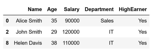
condition_1 = df['Salary'] > 80000
condition_2 = df['Age'] < 40
young_with_high_salary = df[condition_1 & condition_2]
The code above will store the following DataFrame inside the young_with_high_salary variable:
It is possible to inform Pandas that it is sufficient if only one of the multiple conditions is satisfied. This is done in a similar way to how we use the & logical operator to tell Pandas that both conditions need to be satisfied. For instance, let's select those individuals who are either older than 50, work in IT, or both. To do so, we will use the | logical operator:
# Select those that are older than 50
# or work in the IT department
# or both
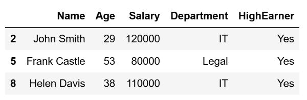
condition_1 = df['Age'] > 50
condition_2 = df['Department'] == "IT"
old_or_in_IT = df[condition_1 | condition_2]
The code above will store the following DataFrame inside the old_or_in_IT variable:
Finally, let's demonstrate how negation can be used. For instance, let's select all those that do not satisfy the conditions we set in the previous example i.e. they can't be older than 50 or work in the IT department, or both. Using the negation logical operator ~ can be achieved by running the following code:
# Select those that are not older than 50
# or that don't work in the IT department
# or both
condition_1 = df['Age'] > 50
condition_2 = df['Department'] == "IT"
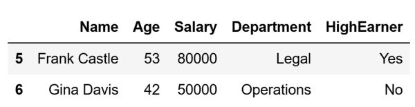
young_or_not_in_IT = df[~(condition_1 | condition_2)]
The code above will store the following DataFrame inside the young_or_not_in_IT variable:
As can be seen, the result is exactly the opposite compared to the one in the previous DataFrame, the old_or_in_IT DataFrame, by negating the conditions we used to create it.
How Do We Filter Data Using Custom Functions?
The most flexible way of filtering data is by creating custom functions and applying them to our data using the apply method. The apply method in Pandas is what we use to apply a function along an axis of a DataFrame, or even on a particular Series. Using the apply method we can apply functions that perform row or column-wise operations, element-wise transformations, aggregate data, and even more.
In the context of filtering, the apply method is used to apply a custom function to each row or column. That function needs to return a Boolean value for each row and column i.e. it needs to return a Boolean Series that we can then use to index the DataFrame.
Let's take a look at an example. Imagine you want to filter out rows where the ratio of Age to Salary is below a certain threshold and the Department is IT. To do so, we first need to define a custom function:
# Create a custom function we will apply on our DataFrame
def IT_salary_custom_filter(row):
    age_salary_ratio = row['Age'] / row['Salary']
    return age_salary_ratio < 0.00025 and row['Department'] in ['IT']
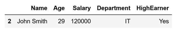
After preparing this function, we can apply it to the data stored in our DataFrame using the apply method. To use this as a method for filtering, we will simply use the result of applying the function on our data as the condition:
# Filter data using the custom function
condition = df.apply(IT_salary_custom_filter, axis=1)
custom_filtered_df = df[condition]
The code above will store the following DataFrame inside the custom_filtered_df variable:
As can be seen above, only John Smith satisfies the criterion set by the custom function. This is why we get a DataFrame that consists of a single row as our final result.
In conclusion, this article provides an in-depth exploration of data filtering in Pandas, a critical skill for effective data analysis. In Pandas, we explored diverse filtering techniques, starting with simple single-condition filters and progressing to more complex multi-condition filters using logical operators. Additionally, we delved into employing custom functions for highly flexible and tailored data filtering.

