For a long time, Pandas has been the go-to library for data analysis and processing in Python. Its popularity comes mainly from its ease of use. Compared to earlier tools, it also offers better performance and flexibility. However, a newer library called Polars has recently been gaining significant attention. It stands out for its impressive speed and modern design, making it an exciting alternative for data professionals.

• Intro to Pandas: What is Pandas in Python?
  

In this comparison, we’ll explore Pandas and Polars side by side across several key areas. We'll examine how each library handles tasks such as data selection, aggregation, reshaping, and other related operations. This comprehensive comparison is designed to help you understand when and how to use each tool. In many cases, it is not a matter of choosing one over the other. You might even find yourself using both libraries within the same project.

What Are the Fundamental Architectural and Philosophical Differences Between Pandas and Polars  

Before diving into code, it’s important to understand how Pandas and Polars work under the hood. Their architectural and philosophical differences help explain why one might outperform the other in certain tasks. The two libraries differ in:

• Language and Implementation
• Memory Model
• Execution Type
• Indexing
• Concurrency 

How Do Pandas and Polars Differ in Language and Implementation

Pandas is implemented in Python, with critical components written in C through NumPy. In contrast, Polars is written in Rust.

• The Ultimate Python Pandas Cheat Sheet

Rust is a modern low-level programming language known for delivering performance similar to C. It also offers powerful safety and concurrency features. Thanks to these, Polars can efficiently use all CPU cores in parallel. 

Pandas operations, on the other hand, typically run on a single thread by default. This can quickly become a bottleneck when working with large datasets. 

How Do Pandas and Polars Differ in Their Memory Model

Pandas stores data in memory using NumPy arrays. These are contiguous blocks of memory that hold data from each column of a dataset. This approach works well for numeric data but can be less efficient for strings or mixed types. 

Polars uses the Apache Arrow columnar memory format, which is becoming a standard for analytical workloads. Arrow’s format is more efficient in terms of memory use and cache performance. As a result, Polars often requires less memory to handle the same data. 

• How Is Pandas Enhancing Data Analysis in Excel

Thanks to this optimized memory representation, Polars typically needs only about two to four times the dataset size in RAM during operations. Pandas, by comparison, might require around five to ten times as much. 

To be fair, Pandas has also recently introduced support for Apache Arrow. They recognized it as an efficient memory format for data storage.

How Do Pandas and Polars Differ in Their Execution Type

By default, Pandas uses eager execution. This means it performs each operation immediately and returns the results right away. 

Polars, on the other hand, support both eager and lazy execution. In lazy mode, Polars doesn't execute operations immediately. Instead, it builds up a "query plan," which is a graph of operations to be performed. 

The query plan only runs when the user explicitly requests the results. This approach allows Polars' optimizer to analyze the plan before execution. It can then reorder operations, skip unnecessary steps, and apply other optimizations to improve efficiency. 

Pandas does not have a built-in query optimizer. It performs operations one by one and always returns the result immediately.

How Do Pandas and Polars Differ in Their Approach to Indexing

Pandas uses an index to label each row. These labels can be numbers, dates, or strings. It even supports multi-level indices for hierarchical data. In contrast, Polars does not have an implicit row index. Each row is identified simply by its integer position. This enables Polars to treat data frames as plain tables with rows and columns, similar to SQL tables. 

Pandas allows you to set and manipulate indices, which can often be very useful. Ultimately, whether you prefer working with indices or not is a matter of personal preference. It does not significantly affect the overall workflow.

How Do Pandas and Polars Handle Concurrency and Parallelism

As mentioned previously, Polars can use all CPU cores in parallel. This makes it much faster for large datasets or computationally intensive tasks. Polars automatically parallelizes many operations and uses vectorized operations under the hood. 

Pandas also benefits from vectorization through NumPy. However, some Pandas operations, especially those involving different types of looping, cannot fully utilize modern hardware.  That said, Pandas has a much more mature ecosystem than Polars. Because of this, you can always find ways to speed up your workflows. For instance, cudf.pandas from Rapids enables users to run operations on the GPU when possible, falling back to CPU otherwise. It handles synchronization under the hood to optimize performance.

What Are the Core Container Objects in Pandas and Polars

After covering the key conceptual differences, let’s take a closer look at the core container objects used by both libraries. We will explain what these containers are, how they are stored in memory, and how to create them in Pandas and Polars.

What Are the Core Container Objects in Pandas

In Pandas, every dataset is stored in either a Series (1-D) or a DataFrame (2-D), both of which are indexed by an immutable Index object. 

A Pandas Series is a 1-D labelled array capable of holding any type of data. It carries its own Index, which provides row labels. Under the hood, it is essentially a NumPy array, so all elements are treated as if they share the same data type. In practice, Pandas Series objects often serve as the columns in a tabular dataset.

A Pandas DataFrame is a 2-D labelled data structure. It consists of multiple columns, each of which can hold a different data type. In essence, a DataFrame is an ordered dictionary of Pandas Series objects that all share the same index. DataFrames are mutable. You can freely add or remove columns and rows. Because each column can have a different data type, the underlying memory blocks may be contiguous within a column but not across the entire Dataframe. This can lead to variable cache efficiency during computation.

• How to Add Columns to a Pandas DataFrame

The Index is an immutable sequence used for indexing and alignment. By default, every DataFrame and Series operation aligns on the index. This enables label-based joins and arithmetic. However, the index adds memory overhead and can sometimes surprise beginners.

What Are the Core Container Objects in Polars

To understand how Polars work, it is important to become familiar with  the following object types:

• Series
• DataFrame
• LazyFrame

A Polars Series is a single-typed column backed by an Apache Arrow buffer. This is the same in-memory format used by Spark, DuckDB, and many other data engines. Arrow stores values contiguously and keeps separate “child” buffers for offsets, validity bits, and variable-length data like strings. This design allows Polars to slice or filter data without copying it. 

Here is how you create an example Polars Series:

import polars as pl

# Create example series

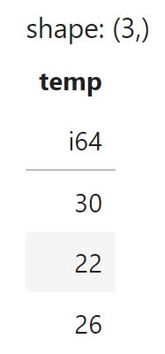
s = pl.Series("temp", [30, 22, 26])

The code above will create the following Series:

A Polars DataFrame is essentially an ordered map of Polars Series objects that share the same number of rows. Each column is stored in its own Apache Arrow buffer. This means scanning a single column only touches the relevant bytes. This design is excellent for analytics workloads, where you often read just a few columns out of dozens. DataFrames can be easily converted into LazyFrames if we wish to switch from eager to lazy evaluation. 

Here is how to create an example DataFrame: 

import polars as pl

# Create example DataFrame

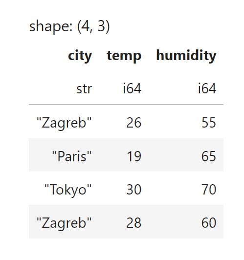
df = pl.DataFrame({
    "city": ["Zagreb", "Paris", "Tokyo", "Zagreb"],
    "temp": [26, 19, 30, 28],
    "humidity": [55, 65, 70, 60],
})

The code above will create the following DataFrame:

Naturally, you can create a DataFrame not only from scratch but also by loading data from a CSV file or other file types. The methods to do this are very similar to those in Pandas. For instance, to load in data from a CSV file into a DataFrame, we would run:

import polars as pl

# Eager read a file
df = pl.read_csv("dataset.csv")

A Polars LazyFrame holds a DAG of query steps instead of immediate results. This approach is similar to how Spark DataFrames or SQL planners operate. Before execution, the optimizer rewrites the graph to improve performance. For example, it pushes filters below joins, drops unused columns, fuses multiple kernels, and enables on-disk streaming to handle out-of-core data efficiently. 

• Intro to Pandas: What is a Pandas DataFrame and How to Create One

To create a LazyFrame from an existing DataFrame, we use special functions such as df.lazy(). Other operations allow us to materialise the result after execution by moving the data into memory or writing it directly to disk. The primary function for this is collect(). 

We can also create LazyFrames directly from different types of files, including CSV files. For instance, you can create a LazyFrame from a CSV file by running the following code:

import polars as pl

# Lazy read a file
lf = pl.scan_csv("dataset.csv")

If I try to access the data directly, I will only get a DAG representation, not a DataFrame with actual data. Therefore, to access information, I need to use the collect() function. For instance, to access the first five rows, I can combine the head() method with the collect() method like this:

import polars as pl

# Lazy read a file
lf = pl.scan_csv("dataset.csv")
lf.head().collect()

How Do Data Selection and Column Operations Work in Polars

We discussed indexing and selecting data earlier, but that initial overview was mostly conceptual. Now, it's time to demonstrate how we approach row and column selection, slicing, and indexing in Polars through practical examples.

• How to Select Data Using .loc in Pandas
• How to Select Data Using .iloc in Pandas

Polars does not have .loc or .iloc methods. Instead, it uses a simpler indexing model because there is no concept of a labeled row index. The common ways to select data in Polars include:

• Column Selection
• Row Selection by Position
• Filtering
• Selecting by Numeric Ranges or Conditions

To simplify data selection and manipulation, we use two powerful methods:

• select()
• with_columns()

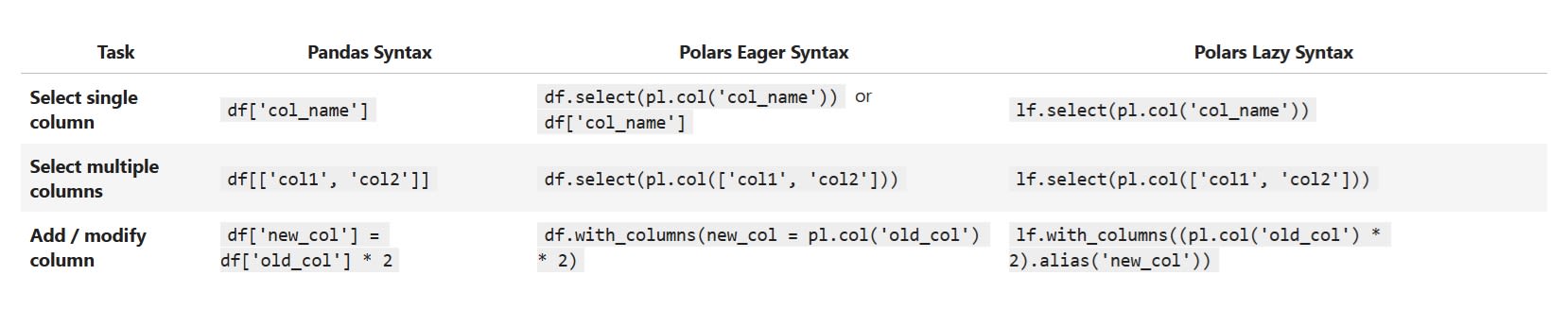
The select() method is used to build a view (or projection) containing only the columns or expressions you specify. For example, you use it when you want to extract and return just one column. 

On the other hand, with_columns() method is designed to add or replace columns while keeping the rest of the DataFrame intact.

These two methods create what we call contexts. They define the scope of our operations and specify which part of the data we want to affect. Inside these contexts, we use expressions, which are the actual operations performed on data. Here are the most common and basic column operations in Polars:

As shown in the examples above, when selecting columns, we can use syntax that resembles Pandas. However, this can lead to bad habits because most operations in Polars must be performed using expressions executed in a certain context. Therefore, it is better to get used to performing operations in this way.

Beyond the basic operations mentioned earlier, Polars also supports many more advanced capabilities. The most commonly used operations include:

• filter()
• sort()
• drop()
• drop_nulls()
• fill_nulls()
• unique()

Let’s load some data to demonstrate how these operations work in practice.

import polars as pl

# Create a DataFrame
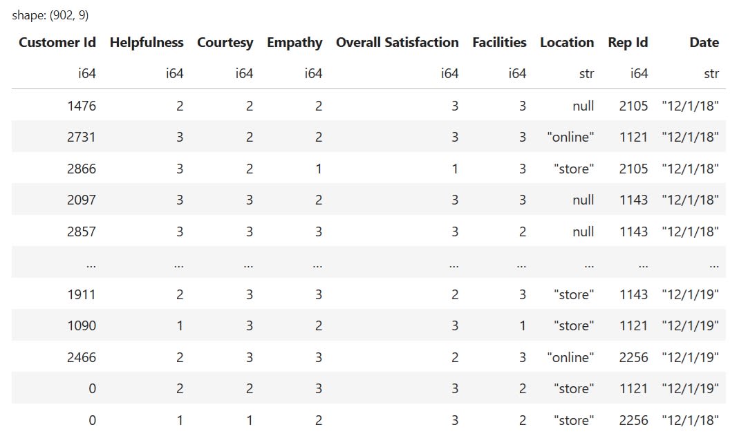
df=pl.read_csv("https://edliteradatasets.s3.amazonaws.com/survey_sample.csv")

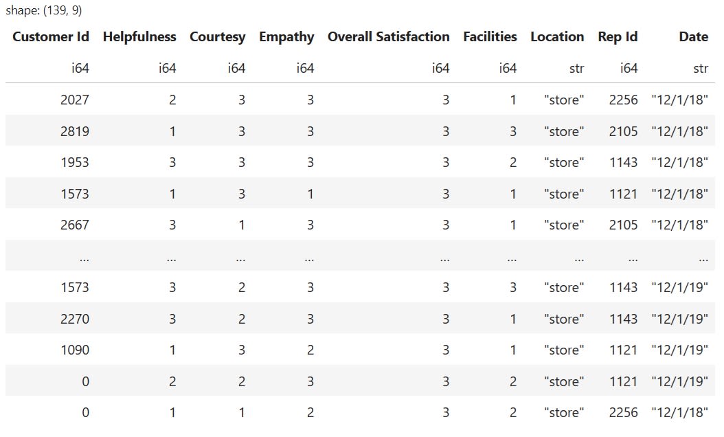
This is what the DataFrame we just loaded looks like:

In Polars, we use the filter() method to keep only the rows that match a specific condition. For instance, the following code filters rows where the value in the "Location" column is "store". It also requires the value in the "Overall Satisfaction" column to be greater than two:

# Filter based on multiple conditions
df.filter(
    (pl.col("Location") == "store") &
    (pl.col("Overall Satisfaction") > 2))

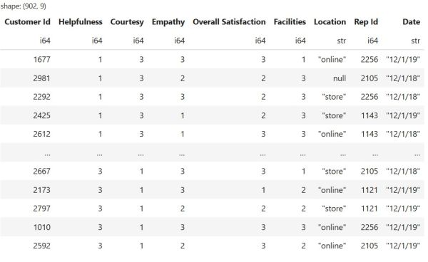
The code above will return the following result:

The sort() method allows us to sort data in a particular order. Its syntax is very similar to that of Pandas. For example, to sort based on two columns, you can use the following code:

# Sort based on two columns
df.sort(["Helpfulness", "Courtesy"], descending=[False, True])

The code above will generate the following result:

The drop() and drop_nulls() methods are used to drop columns and rows from a DataFrame. To be more precise, we use drop() when we want to remove a column. Here is how it works:

# Drop the "Facilities" column
df = df.drop("Facilities")

This will remove the "Facilities" column from our DataFrame. If we want to remove all rows that contain a missing value, we can use the drop_nulls() method like this:

# Drop any row with a missing value in any column
df = df.drop_nulls()

Filling in missing data with fill_null() works a little differently. We need to specify what to replace the missing values with. This can be a scalar, the column mean, the most frequently occurring, or many other options. For instance, in our example DataFrame, the "Location" column has missing data. Since this column contains non-numerical data, it makes the most sense to replace the missing values with the value that appears most frequently in the column. To do this, we can run the following code:

# Replace missing values with with the most frequently occurring value
df=df.with_columns(
      pl.col("Location").fill_null(pl.col("Location").mode().first()
)

Finally, to check for duplicates, we use the unique() method. Polars handles duplicates similarly to SQL. It allows us to detect, keep, drop, or summarise duplicates using several verbs that work the same way in both eager DataFrame mode and delayed‐execution LazyFrame mode. For instance, if I want to remove duplicates based on the "Customer Id" and "Rep Id" columns, I can use the unique() method like this:

# Remove duplicates from the "Customer Id"
# and the "Rep Id" column
df.unique(
    subset=["Customer Id", "Rep Id"],   # None = all cols
    keep="any",                   # 'any' | 'first' | 'last' | 'none'
    maintain_order=True           # keep row order if wanted
)

How Do Merging and Joining Data Work in Polars 

Real-world data work often requires merging two datasets. In Polars, we use the join() method to perform this merging. The method supports different types of  join operations, such as: 

• inner join
• left join
• right join
• outer (full) join

Let’s create two DataFrames to demonstrate how these operations work:

import polars as pl

# Create first DataFrame

countries = pl.DataFrame({
    'Letter': ['a', 'b', 'c', 'd', 'n', 'o'],
    'Country': ['Andorra', 'Belgium', 'Croatia', 'Denmark', 'Niger', 'Oman']})

# Create second DataFrame

capitals = pl.DataFrame( {
    'Name': ['Andorra', 'Denmark', 'Spain', 'Portugal'], 
    'Capital': ['Andorra la Vella', 'Copenhagen', 'Madrid', 'Lisbon']
} )

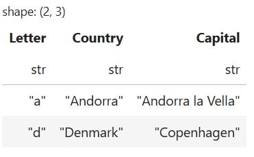
Merging data in Polars uses syntax very similar to Pandas. The only differences are in the names of some arguments. For instance, to perform an inner join, you would use the following code:

# Perform an inner join
countries.join(capitals, left_on="Country", right_on="Name", how="inner")

The code above will produce the following result:

To perform other join operations, simply change the value of the how argument from "inner" to one of the following options: "left", "right", or "full".

How Does Data Aggregation Work in Polars

Both Pandas and Polars excel at grouping data and computing aggregate statistics. Polars provides similar functionality to Pandas, but with a different style. Its API is very expression-oriented, which means you often pass in pl.some_function() instead of just a string like "mean" as you would in Pandas. 

• How to Do Time Series Analysis With Pandas

At first, this might seem like extra boilerplate code. However, this design avoids ambiguity and unlocks the full power of Polars' expressions. For example, it allows you to perform filtering or arithmetic within the aggregation when needed.

There are two main ways of aggregating data in Polars:

• group_by()
• pivot()

What Is the group_by() Method in Polars

In Polars, the group_by() operation is a powerful and efficient way to aggregate data. It partitions the DataFrame into groups based on shared key values. Then, it performs specified aggregations within each group and returns one summary row per group. 

Because this process compresses rows without expanding the schema, it remains computationally efficient. Polars supports group_by() in both eager and lazy execution modes. It can stream data in chunks and allows multiple aggregations to be pipelined in a single pass. 

For these reasons, group_by() is the recommended method for statistical summarization and feature engineering in Polars. 

To use it effectively, two parameters must be defined: 

• by - specifies the column(s) used for grouping.
• agg - outlines the aggregation(s) to apply within each group.

Let’s create an example DataFrame to demonstrate how to aggregate data using group_by():

import polars as pl

# Create sample data
data = {
    "order_id": [1, 2, 3, 4, 5, 6, 7, 8, 9, 10],
    "region": ["North", "South", "North", "East", "West", "South", "West", "North", "East", "South"],
    "product_category": ["Electronics", "Books", "Electronics", "Home Goods", "Books", "Books", "Electronics", "Home Goods", "Books", "Home Goods"],
    "sales": [250.0, 45.5, 300.0, 120.0, 35.0, 60.0, 450.0, 85.0, 55.5, 95.0],
    "quantity": [2, 3, 1, 5, 2, 4, 1, 3, 3, 4],
    "order_date": [
        "2023-01-15", "2023-01-16", "2023-02-10", "2023-02-12", "2023-03-05",
        "2023-03-06", "2023-04-20", "2023-04-21", "2023-05-18", "2023-05-19"
    ]
}

# Create DataFrame
df = pl.DataFrame(data)

# Convert string dates to Polars Date type for time-based aggregations
df = df.with_columns(pl.col("order_date").str.to_date())

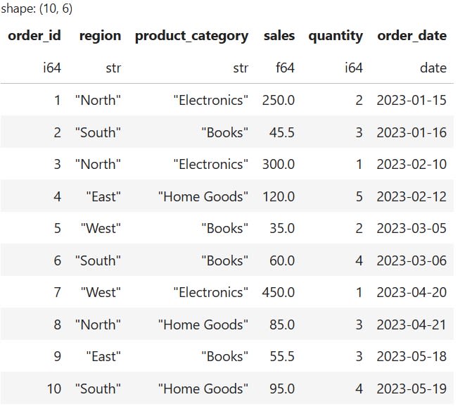
Here is what the DataFrame looks like:

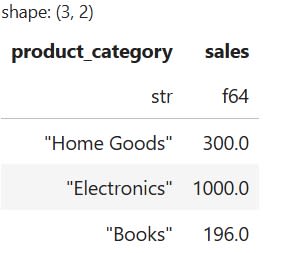
Suppose I want to group data based on the product_category column. This allows me to calculate the total sales for each unique category. To achieve this with group_by(), I can use the following code:

# Group by product_category and calculate the sum of sales
total_sales_by_category = df.group_by("product_category").agg(pl.sum("sales"))

The code above creates the following result:

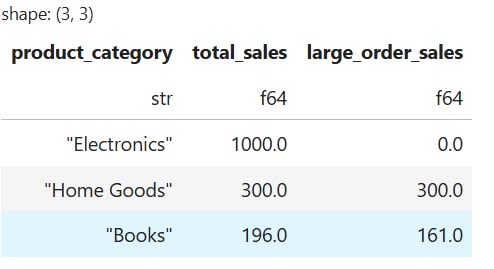
Naturally, we can perform more complex operations using group_by() to analyze specific subsets of our data. For instance, suppose I want to group by category, but also compare total sales with sales from large orders. In this case, I need to both aggregate and filter the data simultaneously. Fortunately, the group_by() method allows me to do exactly that by running the following code:

# Group by category and calculate total sales vs. sales from large orders

conditional_sales = df.group_by("product_category").agg([
 pl.sum("sales").alias("total_sales"),
 pl.col("sales").filter(pl.col("quantity")2).sum().alias("large_order_sales")
])

The code above will generate the following result:

What Is the pivot() Method in Polars

In Polars, the pivot() method serves a different purpose than group_by(). It is primarily used for reshaping data rather than summarizing it. When you use pivot(), it transforms the DataFrame by turning unique values from a specified pivot column into new column headers. It then fills the resulting matrix using an aggregation function, such as sum or mean. 

This process widens the table horizontally. Polars needs to identify all distinct values in the pivot column beforehand to set up the correct schema. Because of this requirement, pivot() is only available in eager execution mode. The schema cannot be determined lazily. 

Conversely, the unpivot() function reverses this transformation. It converts wide data into a taller and narrower format. Together, pivot() and unpivot() provide flexible ways to reshape data structures in Polars.

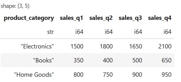
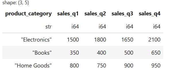
Let’s demonstrate how these two methods work by first creating an example DataFrame. By default, a newly created DataFrame will be in a "wide" format.

import polars as pl

# Create a sample "wide" DataFrame
data = {
    "product_category": ["Electronics", "Books", "Home Goods"],
    "sales_q1": [1500, 350, 800],
    "sales_q2": [1800, 400, 750],
    "sales_q3": [1650, 500, 900],
    "sales_q4": [2100, 650, 950]
}

# Create DataFrame
wide_df = pl.DataFrame(data)

This is how our DataFrame looks:

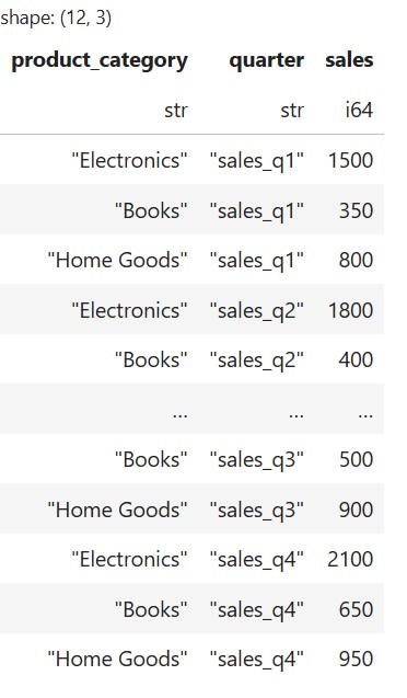
When sales data is stored with each quarter in a separate column, it creates a "wide" format. This format is not ideal for aggregations or time-series plotting. To make the data easier to analyze, it's best to transform it into a "long" format. In this structure, the separate quarter columns are combined into a single column representing the quarter. Another column holds the corresponding sales figures. This format simplifies tasks like grouping, filtering, and visualizing trends over time. 

• How to Filter a Data Set using Pandas

To change the format of our data, we will use the unpivot() method:

# Unpivot the DataFrame to a long format 

long_df = wide_df.unpivot(
        index="product_category",
        on=["sales_q1", "sales_q2", "sales_q3", "sales_q4"],     
        variable_name="quarter",             
        value_name="sales
)

The code above will produce the following DataFrame:

Most of the time, you will encounter data that needs to be unpivoted to be in the optimal format for analyzing and processing. However, if you find yourself with data in a "long" format but want to convert it back to "wide", you can use the pivot() method. 

For instance, to transform our data back to its original wide format, we can run the following code:

# Pivot the long DataFrame back to a wide format

pivoted_df = long_df.pivot(
    values="sales",
    index="product_category",
    on="quarter"
)

The code above will produce the following result:

Both Pandas and Polars offer compelling advantages for data analysis. The choice between them depends largely on your specific needs and constraints. Pandas remains the mature, battle-tested option with an extensive ecosystem and an intuitive API familiar to most Python users. 

• Building a Video Editing App in Python: How to Create a UI with Streamlit (Part 1)

Polars, however, brings modern performance optimizations, superior memory efficiency, and powerful lazy evaluation capabilities that can significantly speed up analytical workflows, especially with larger datasets. 

In this article, we focused on the basics of using Polars for fundamental data manipulation tasks. We also highlighted key differences from Pandas to help bridge the gap between the two libraries.