


In the previous article of this series, we began discussing generative models in AI. These models constitute a class of AI algorithms designed to generate new data samples resembling those of a given set of data. Variational Autoencoders and Generative Adversarial Networks were the two models we covered in the previous article. These algorithms are commonly used in the field of Computer Vision to generate new, synthetic data. In this article, we will build upon the foundations of the previous article and introduce Diffusion models. They are the newest addition to the family of generative models in the field of Computer Vision. We will cover the fundamental concepts and delve deeper into the architecture in the following article.
What is Diffusion
Diffusion models are a type of generative model, similar to VAEs and GANs. They are relatively new but have already shown impressive results in generating highly diverse images of extremely high quality. In that regard, they are considered to be at least at the same level as modern GANs. Moreover, they can even outperform them in some aspects. The working principle of these models is inspired by the physical process of diffusion.
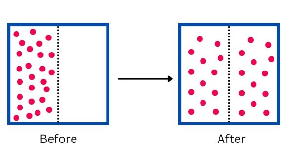
Diffusion is a natural physical phenomenon where particles and energy move from a region of higher concentration to that of lower concentration. At the microscopic level, diffusion is driven by the random and chaotic movement of particles. Such a phenomenon is referred to as Brownian motion. This process takes place as systems seek to reach equilibrium, a state where particle concentrations are evenly dispersed throughout the system.
There are many examples of diffusion you can witness daily. For instance, when you cook something the aromatic molecules are highly concentrated at first around the food. As time passes, these molecules start to spread out and move through the air to areas of lower concentration. This is why you can detect the cooking smell even from a distance. The concept of diffusion in AI models is metaphorically similar to the physical process of diffusion.
Article continues below
Want to learn more? Check out some of our courses:
What Is Diffusion in the Context of Machine Learning
Diffusion models in Machine Learning function by learning how to reverse a diffusion process. This process begins with a distribution of random noise and then gradually transforms it into a structured image. In simpler terms, they learn to ''destroy'' training data by adding Gaussian noise, and then reconstruct the data from the ''destroyed'' version. Training a model in such a way allows us to later pass randomly sampled noise to the model and constructs a new data point for us. The process itself can be broken down into two main phases:
- Forward diffusion
- Reverse diffusion
What Is Forward Diffusion
Forward diffusion is the process of deconstructing some original data point. In the context of Computer Vision, this would be an image, in the form of random noise. In the context of working with images, noise is random pixels that do not follow any pattern or structure. An analogy would be the static you see on an untuned TV channel. Noise is added to our original image through multiple iterations. In each iteration, we add a small amount of noise, for example. random pixels until we reach a state that is referred to as "pure noise". At this point, we can no longer recognize the original image.
A degree of randomness is introduced at each step as a byproduct of the noise addition process. However, the entire process is still designed to be both predictable and reversible. This is possible because of the precise knowledge of the amount and nature of noise added at each step. That information makes the reverse diffusion process possible and enables the reconstruction of our data from the pure Gaussian noise generated at the conclusion of the forward diffusion process.
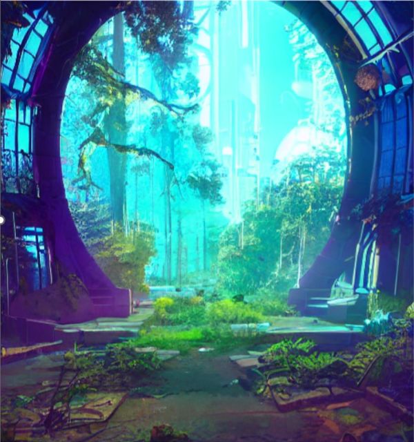
Let us take a look at a simple example. Imagine that we have the following image in our training set, and we want to deconstruct it using our diffusion model.
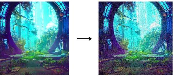
In the first few iterations, the added noise only makes the image look slightly more grainy.
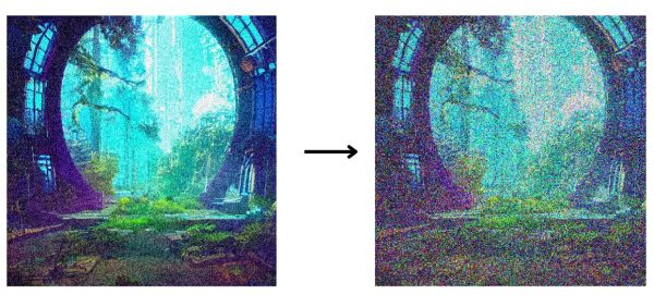
However, as the number of iterations increases, the accumulating noise begins to distort the image more and more.
After many iterations, we reach a state referred to as "pure noise". At this point, we can no longer discern the original image because it has been completely deconstructed into noise.
Mathematically speaking, forward diffusion can be described as a Markov chain. A Markov chain is a mathematical system that undergoes transitions from one state to the next. That consists of a finite number of possible states. The main characteristic of a Markov chain is that there is no concept of ''memory'' in the chain. This means that the probability of transitioning to any future state from the current one depends only on the current state, instead of the previous one.
In the context of diffusion models, the addition of noise performed in each step of the forward diffusion process can be viewed as a transition in a Markov chain. The current state, represented by an image with a certain level of noise, is solely influenced by the image resulting from the addition of noise in the previous step. In simple terms, when adding noise to the image, you are adding it to the version of the image that resulted from the previous step. This characteristic makes the forward diffusion process computationally efficient. It greatly simplifies both the modeling of the noise addition and the subsequent reversal process performed during the reverse diffusion step.
- How to Use Machine Learning to Automate Tasks
- What Is The Difference Between Machine Learning and Artificial Intelligence?
What Is Reverse Diffusion
The reverse diffusion process aims to reverse what was done during forward diffusion. By going through multiple steps, data is reconstructed from a noisy state back to its original form or a new coherent form. This process is especially important because, in the context of diffusion models, performing inference with a trained model is equivalent to performing reverse diffusion.
We begin with a sample of noise, a random and unstructured input, and proceed through multiple steps where we gradually remove noise from the sample. As we proceed backward through the iterations, our image will transition through states of decreasing levels of noise. This continues until we either reconstruct the original image or construct a new, plausible image. The details behind reverse diffusion are highly complex. However, that will be explored in the subsequent article in this series, the one about the math behind diffusion models.
What Is the Difference Between Reconstructing Original Data versus Creating Original Data
As mentioned previously, at the end of the reverse diffusion process, we may reconstruct the original image from the forward diffusion process or generate an entirely new image. For example, if we train our model on a dataset that contains many cat images, the model will be able to generate an image of a realistic cat. However, such an image would be completely new and would not exist in the training set of images. We influence the outcome by providing the correct information to the model. In addition, we can do that by telling the model how creative it should be.
A typical input that can be used to guide the model during inference is a text prompt. This is something frequently used when working with images. The prompt usually contains a set of constraints or guidelines that show the model about the desired end result. This could include elements such as the subject of the image, the style, the color scheme, or even the presence of certain objects or themes. In fact, modern diffusion models can even take in some other image as input. Afterward, it can be used as a reference to extract the overall topic of the image we want to create, the style, etc.
Our input is unable to specify every detail of the final image. Therefore, the model uses its training to fill in the blanks. It draws on patterns, textures, and relationships acquired during training from a vast array of images. This is how it can generate complex and coherent images even from simple or abstract prompts.
Finally, when setting up the creation process we can also define how creative we want the model to be. During training, the model is exposed to a wide variety of images. This is where it learns the common patterns and rules of image composition. Through extensive training, the model gains an understanding of typical image characteristics and what renders them visually appealing or coherent.
While the model will attempt to adhere to the input prompt we provided, it also has the freedom to introduce new elements or interpret the prompt in unique ways. This is where the model's creativity comes into play. The balance here is crucial. On the one hand, an abundance of adherence to the input can result in dull and repetitive images. On the other hand, an abundance of creativity can lead to images that are not in alignment with the user's intentions.
Controlling the degree of creativity in a diffusion model, for example, those used for image generation, involves tweaking certain parameters and aspects of the model's operation. These two parameters are:
- Temperature
- Sampling method
In the context of AI, particularly generative models, "temperature" is a hyperparameter that controls the randomness in the model's output. A low-temperature value results in less randomness. In other words, the model is more likely to choose high-probability options, resulting in more predictable and conservative outputs. This is similar to the model of playing it safe, sticking closely to the acquired patterns during training. A high temperature increases randomness. The model is more likely to sample less probable options, resulting in more varied and creative outputs. This can sometimes lead to surprising or novel combinations, but also to less coherent or relevant results.
Sampling methods refer to the techniques used to generate outputs from a probability distribution. For example, when dealing with images we would refer to the denoising process as sampling. This means that the method we use to denoise would be called our sampler. Different samplers can affect the characteristics of the generated images. Therefore, the choice of a sampler is often a trade-off between speed, image quality, and the level of creativity or variation in the outputs. In practice, the selection of a sampler may depend on the specific requirements of a project or experiment. As a result, deciding which sampler to use is quite a complex topic. We will further delve into it in the following article in this series.
In practical applications, diffusion models are usually not employed for reproducing original data, as there are other models more effectively designed for this purpose. However, diffusion models excel in generating new data, particularly images. Here they surpass other models in terms of the quality and diversity of the output they produce.
- 5 Machine Learning Security Risks You Should Watch Out For
- What Are the Most Common Types of Machine Learning Styles?
In this article, we explained the basic workings of diffusion models. We clarified what diffusion is, and how we implement it through forward diffusion and reverse diffusion. Moreover, we tackled the topic of data reconstruction versus creating new data. In the following article in this series, we will continue building upon this. Stable Diffusion, an especially specific type of diffusion model will be covered. Such a model is one of the most advanced diffusion models designed for the creation of new original images.

