


Table of Contents
"Garbage in, garbage out" is a famous saying in the machine learning community. It means that, whenever you train any model, whether it be a deep learning model or just a statistical model, you always need to make sure that you are feeding it good data. Bad results are inevitable if you use the wrong data, even if you do pick the right model for the job. Many different data preprocessing techniques have been developed to make sure that even if you don't have access to ideal data, you can still get the most from what you have at your disposal. These data preprocessing techniques vary from task-to-task and are as important as the model you plan on using.
You will often hear people refer to the data preprocessing step as "image augmentation." Image augmentation is what you do before you feed your image data into a computer vision model. In this article, I will talk about what image augmentation is, what are common image augmentation techniques, and how to implement them in Python.
This is the first article in a series of articles that will prepare you to integrate an image augmentation pipeline into your current pipeline to improve the results you get from your models.
Why Use Image Augmentation?
Data preprocessing will include various steps that modify your data before you use it for training your models. While image augmentation can't be considered data preprocessing if you look at it from that angle, it serves the same purpose to modify in some way the data you plan on training your model on. In the case of image augmentation, that means adding new, artificially created images to the dataset of images you plan to train your model on.
As everyone working in the field of machine learning knows, deep learning models are very "data hungry." Researchers are constantly working on creating models that can be trained on small quantities of data, but even those small quantities of data are usually measured in the thousands. This often leads to one very simple problem: even if you have a quality model at your disposal, you don't have enough quality data to train it on. Many fields use computer vision and greatly suffer from the lack of data.
- What Questions Can Machine Learning Help You Answer?
- Automation with Machine Learning: How to Use Machine Learning to Automate a Task
One good example of low quantity data affecting quality data is in the medical field.
Training models to solve some typical medical problems, such as segmenting tumors on a CT image, is very hard. For each image, the patient needs to give consent because each image is considered private data. Finding enough patients willing to let others look at their confidential information is problematic, and usually leads to researchers working with datasets that are lacking in terms of data quantity. Of course, this isn't a problem that solely plagues the field of medicine. Many other fields often find it hard to gather as much data as they need to create a dataset of high quality.
This lack of data can, to some degree, be remedied using image augmentation. Getting more real data is still preferred and will always be the best thing one can do when a dataset isn't big enough. In those cases where you can't do it in a reasonable time frame, you can use image augmentation.
Image augmentation is so effective, people use image augmentation even when they do have high-quality datasets because the same artificially created images that help you increase the accuracies when you train on smaller quantities of data help you further increase accuracy when you train on larger quantities of data.
- How can Emotional Artificial Intelligence Improve Education
- How to Detect Emotions in Images Using Python
Nowadays, most research papers that cover topics on deep learning in computer vision introduce at least basic augmentation methods when training the model that the paper is presenting. This trend can be easily followed by looking at the most prominent computer vision deep learning models through history.
AlexNet, Inception, ResNet, and many more have all included image augmentation techniques when training their models. The importance of image augmentation is so great that Google even created an algorithm called AutoAugment in 2018. AutoAugment’s sole purpose is to pick the best possible set of augmentations to use for a particular set of data.
How Image Augmentation Works
Image augmentation is the process of creating artificial images from existing ones, that can be used as part of your training dataset. In other words, taking an original image from your dataset and changing it in some way. There are various changes you can introduce, but all of them will yield the same result of an image that is good enough for your model to train on, yet different enough that it can't be considered a duplicate of the original image.
Though useful, the situation isn't quite as simple as it sounds. Creating artificial images and using them for training doesn't necessarily need to lead to better results. In fact, when used improperly, image augmentation can even decrease the accuracy of a network. However, there are guidelines that, if followed, will increase the odds of good results.
In most articles, you will find that image augmentation techniques are either not separated into categories at all, or are only separated into position and color augmentation techniques. Separating augmentation techniques this way is somewhat of an oversimplification. If you want to be precise, it is better to look at the process of creating a new image. Depending on how a transformation changes the original image to create a new image, you can separate the different transformations you use into:
- Pixel-level transformations
- Spatial-level transformations
In this article, I will cover the simpler of the two types of transformations, pixel-level transformations. In a future article, I will cover spatial-level transformations, and how to build image augmentation pipelines.
Article continues below
Want to learn more? Check out some of our courses:
How to Use the Albumentations Library
There are numerous ways of including an image augmentation pipeline in your machine learning project. Your library of choice will be Albumentations. While the easiest way is to use one of the libraries that were created for performing various tasks with images (e.g., PIL), Albumentations is the better choice. Albumentations not only allow you to transform images but also make it very easy to create image augmentation pipelines (a topic I will cover more in-depth in the following article in this series). Other libraries, such as Torchvision, are also good choices but are limited in their integration options. Torchvision integrates with PyTorch, while Albumentations can integrate with both Keras and PyTorch.
Albumentations is a library in Python specially designed to make doing image augmentation as easy as possible, being specifically designed for augmenting images. Its simple interface allows users to create pipelines that can effortlessly integrate into any existing Machine Learning pipeline. Overall, Albumentations is better optimized than more general computer vision libraries.
Before I cover different transformations, let's install Albumentations. The easiest way to install Albumentations is using Anaconda or pip. If you want to install Albumentations using Anaconda, the code you need to run is:
conda install -c conda-forge albumentations
If you want to install Albumentations using pip, the code you need to run is:
pip install albumentationsIf you plan on installing Albumentations from a Jupyter notebook, don't forget to add the exclamation sign:
!pip install albumentationsPixel-Level Transformations
There are a plethora of different pixel-level transformations offered by Albumentations. Forty-five, to be exact. Of course, some of them are used more often and some are used less often. In this article, I will cover the most commonly used ones. If you are interested in transformations that are not mentioned here, I recommend taking a look at the Albumentations documentation.
The pixel-level transformations used most often are:
- Blur and sharpen
- Histogram equalization and normalization
- Noise
- Color manipulation
Blur and Sharpen
An important concept of image analysis and object identification in images is the concept of edges. These are places where there are rapid changes in pixel intensity. Blurring images is the process of "smoothening the edges." When you blur an image, you average out the rapid transitions by treating certain pixels as outliers. The process functions as if you were passing the image through a low-pass filter, which is usually used to remove noise from an image.
With Albumentations, you can both sharpen and blur your images. Mathematically speaking, what you are doing is selecting a kernel (often called a convolution matrix or a mask) and passing it over an image. This process is called convolution. Depending on which kernels you pass over your images, you get different results. Sharpening gets us the exact opposite effect, but it works much the same. You just pass a different kernel over your image.
Sharpening images is done using the Sharpen operation. Using this transformation, you highlight the edges and fine details present in an image by passing a kernel over it. Then, you overlay the result with the original image. The enhanced image is the original image combined with the scaled version of the line structures and edges in that image.
Blurring images, on the other hand, is done using one of the following operations:
- Blur
- AdvancedBlur
- GaussianBlur
- MedianBlur
It is worth mentioning that the blur you will probably use most often is GaussianBlur. The Blur transformation uses a random kernel for the operation, so the results you get might not be that great.
The GaussianBlur transformation works great because most of the time the noise that exists in an image will be similar to Gaussian noise. On the other hand, if salt-and-pepper noise appears in the image, using the MedianBlur transformation is a better tool.
The AdvancedBlur operation is theoretically the best possible solution if you have enough time to fully customize your blur transformation. It also uses a Gaussian filter but allows you to customize it in detail, so it best suits your needs. However, in most cases, it is better to just stick with the standard GaussianBlur transformation or MedianBlur, depending on the situation, because time spent optimizing your blurring operation is probably better spent on optimizing your model instead. The standard GaussianBlur transformation is good enough in most cases.
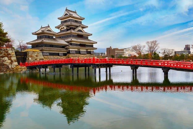
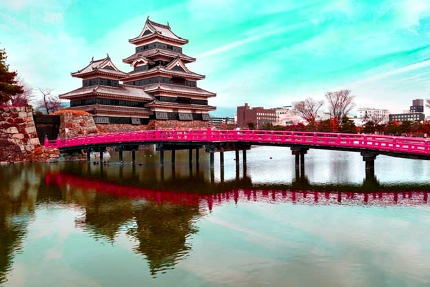
Let's demonstrate the results you get by using the Sharpen, GaussianBlur, and MedianBlur operations on the following image of the Matsumoto Castle in Japan.

Image Source: Matsumoto Castle, https://www.veranda.com/travel/g30083514/beautiful-castles-in-the-world/
Before you apply any transformations, you need to import albumentations and a few other standard image processing libraries:
import albumentations
import cv2
from PIL import Image
import numpy as np
To demonstrate the results of different transformations in a Jupyter Notebook, let's create a small function:
# Create function for transforming images

def augment_img(aug, image):
    image_array = np.array(image)
    augmented_img = aug(image=image_array)["image"]
    return Image.fromarray(augmented_img)
This function will return a transformed image. Take note that you must transform your image into an array before you apply the transformation to it. Once this is prepared, let's load your image, store it into a variable, and display it:
# Load in the castle image, convert into array, and display image

castle_image = Image.open("matsumoto_castle.jpg")
castle_image
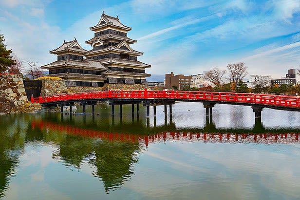
The displayed image is that of the castle shown earlier in this article.
Now that everything is ready, you can apply the transformations to your image and take a look at the results:
Image Source: Matsumoto Castle, https://www.veranda.com/travel/g30083514/beautiful-castles-in-the-world/
Let's first sharpen the image:
# Sharpen the image

sharpen_transformation = albumentations.Sharpen(p=1)
augment_img(sharpen_transformation, castle_image)
As you can see, I left all the parameters of the transformation at their default values except for one. The argument p defines the chance that the transformation will be applied to the image. A p value of 1 means that when you run the code there is a 100% chance that the transformation will be applied.
While this might seem counterintuitive, it makes perfect sense once you see how pipelines work. You can define multiple transformations, define the chance each one will be applied, and then get random combinations of transformations to augment your images. This is something I will expand upon in future articles.
The resulting image is:
Image Source: Matsumoto Castle, https://www.veranda.com/travel/g30083514/beautiful-castles-in-the-world/
If you want to apply the GaussianBlur transformation, you need to run the following code:
# Blur image: Gaussian

gauss_blur_transformation = albumentations.GaussianBlur(p=1)
augment_img(gauss_blur_transformation, castle_image)
The resulting image is going to look like this:
Image Source: Matsumoto Castle, https://www.veranda.com/travel/g30083514/beautiful-castles-in-the-world/
And finally, if you want to apply the MedianBlur transformation, you need to run the following code:
# Blur image: Median

median_blur_transformation = albumentations.MedianBlur(p=1)
augment_img(median_blur_transformation, castle_image)
By applying this transformation, you will get the following result:
Image Source: Matsumoto Castle, https://www.veranda.com/travel/g30083514/beautiful-castles-in-the-world/
Histogram Equalization and Normalization
Histogram Equalization is a contrast adjustment method created to equalize the pixel intensity values in an image. The pixel intensity values usually range from 0 to 255. A grayscale image will have one histogram, while a color image will have three 2D histograms, one for each color: red, green, blue.
On the histogram, the y-axis represents the frequency of pixels of a certain intensity. You improve the contrast of an image by stretching out the pixel intensity range of that image, which usually ends up increasing the global contrast of that image. This allows areas that are of lower contrast to become of higher contrast.
An advanced version of this method exists called Adaptive Histogram Equalization. This is a modified version of the original method in which you create histograms for each part of an image. This allows you to enhance contrast optimally in each specific region of an image.
Albumentations offers a few options to perform histogram equalization:
- Equalize
- HistogramMatching
- CLAHE(Contrast Limited Adaptive Histogram Equalization)
Of the three mentioned, you probably won't use HistogramMatching too often. It is usually used as a form of normalization because it takes an input image and tries to match its histogram to that of some reference image. It is used in very specific situations such as when you have two images of the same environment, just at two different times of the day. On the other hand, the Equalize transformation and the CLAHE transformation are used more frequently.
The Equalize transformation is just a basic histogram equalization transformation. It is often overshadowed by CLAHE.
CLAHE is a special type of adaptive histogram equalization. As a method, it better enhances contrast, but it does cause some noise to appear in the image. Nonetheless, the benefits often outweigh the detriments of using CLAHE, so it is very popular.
To better demonstrate how these methods work, you are going to convert your image into a grayscale image. You can do that using albumentations, since it offers a transformation called ToGray:
# Grayscale image

grayscale_transformation = albumentations.ToGray(p=1)
grayscale_castle_image = augment_img(grayscale_transformation, castle_image)
grayscale_castle_image
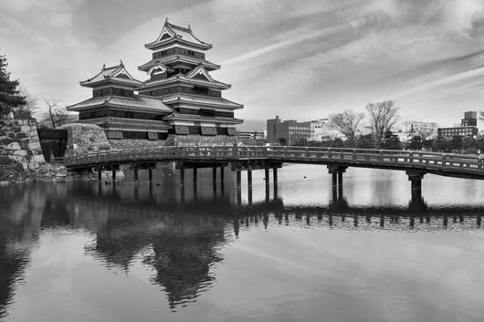
The resulting image will look like this:
Image Source: Matsumoto Castle, https://www.veranda.com/travel/g30083514/beautiful-castles-in-the-world/
Once that's done, you can apply the two transformations.
First, you will apply the standard histogram_equalization method:
# Standard histogram equalization

histogram_equalization = albumentations.Equalize(p=1)
augment_img(histogram_equalization, grayscale_castle_image)
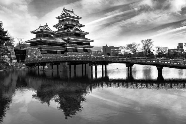
This is what the result of equalizing the histogram looks like:
Image Source: Matsumoto Castle, https://www.veranda.com/travel/g30083514/beautiful-castles-in-the-world/
As you can see, the differences between the darker and lighter hues have been enhanced, which can be noticed especially on the roof of the castle.
Now let's apply CLAHE:
# Standard histogram equalization

CLAHE_equalization = albumentations.CLAHE(p=1)
augment_img(CLAHE_equalization, grayscale_castle_image)
The resulting changes when you apply CLAHE:
Image Source: Matsumoto Castle, https://www.veranda.com/travel/g30083514/beautiful-castles-in-the-world/
CLAHE enhances contrast much better locally. Look at the reflection of the entry to the palace. It is much more pronounced. This would help a model you are training to learn easier and quicker.
Normalization also modifies pixel intensity values and is also used in cases where images have poor contrast due to various reasons. You might be familiar with the term “dynamic range expansion,” which is what normalization is called in the field of digital signal processing.
Put in layman's terms and explained in an example above, normalization allows us to make sure that pixel values in images fall into a certain range. It is particularly useful when you need to make sure that all images in a particular set of data have pixels that follow a common statistical distribution. This is very important for Deep Learning models. When working with neural networks, you want to make sure that all the values that you input into a network fall into a certain range, which is why you normalize data before feeding it to the network.
I won't go into detail right now since normalization is best demonstrated when I explain image augmentation pipelines.
Noise
Noise is something that is, to a certain degree, always present in an image. It is a byproduct of degradation that occurs when you take an image. When an image is taken, the digital signal gets "polluted" along the way, causing random variations in image brightness, and even sometimes in color information.
Even though it might seem counterproductive, sometimes you want to augment your images by adding noise to them on purpose. After all, your model will seldom get images that were taken in perfect conditions or that were previously cleaned. Therefore, teaching a model to recognize something in an image even if that image contains noise is productive, and something you should aim to do.
Albumentations allows you to easily implement:
- GaussNoise
- ISONoise
- MultiplicativeNoise
You'll mostly use GaussNoise, which is a statistical noise, with the same probability density function as that of the normal distribution. It is the noise that occurs in images during image acquisition or image signal transmission. In most situations, it accurately mimics what happens to images in real-life scenarios.
To implement gaussian_noise you need to use the following code:
# Gaussian noise

gaussian_noise = albumentations.GaussNoise(var_limit=(350.0, 460.0), p=1)
augment_img(gaussian_noise, castle_image)
As a side note, I used large values for the var_limit argument to make the noise easier to see on the image. Default values create noise that a machine learning model easily recognizes, but that is not visible to the naked human eye.
The image you get by applying this transformation is:
Image Source: Matsumoto Castle, https://www.veranda.com/travel/g30083514/beautiful-castles-in-the-world/
Color Manipulation
There are different ways of manipulating colors in an image. I already demonstrated one way earlier in this article, when I converted our original image to a grayscale image. That is a very common procedure that a lot of images go through before being fed into a model. If the color itself is not in any way connected to the problem the model is trying to solve, it is common practice to convert all images to grayscale. That’s because building networks that work with grayscale images (single channel images) is much easier than building networks that work with colored images (multi-channel images).
When you do work with images with color, you'll generally manipulate the hue, saturation, and brightness of a particular image.
To perform color transformations in Albumentations you can use:
- ToGray
- ToSepia
- RandomBrightnessContrast
- HueSaturationValue
- ColorJitter
- FancyPCA
ToGray and ToSepia transformations are self-explanatory. ToGray will transform the image into a grayscale image, and ToSepia will apply a sepia filter to the RGB input image.
rand_brightness_contrast (RandomBrightnessContrast) is used very often. It is one of the most commonly used transformations, and not only amongst pixel-level transformations. It does exactly what the name says; randomly changing the contrast and brightness of the input image.
Applying it to an image is done using the following code:
# Brightness and contrast

rand_brightness_contrast = albumentations.RandomBrightnessContrast(p=1)
augment_img(rand_brightness_contrast, castle_image)
The resulting image will look like this:
Image Source: Matsumoto Castle, https://www.veranda.com/travel/g30083514/beautiful-castles-in-the-world/
Since rand_brightness_contrast randomly selects values from a range, if you run the code above, your results might be a bit different. Even if the differences are not easy to recognize with the naked eye, models will still pick up on them.
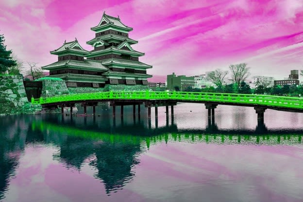
The HueSaturationValue transformation will randomly select values for hue, saturation, and value from a particular range of values. If you want to transform your images using this transformation, you can just run the following code:
# Random hue, saturation, and value

rand_hue_sat_val = albumentations.HueSaturationValue(hue_shift_limit=[50, 60], p=1)
augment_img(rand_hue_sat_val, castle_image)
In this case, I selected extreme values for hue on purpose to demonstrate the changes this transformation can make to the original image.
The resulting image will look like this:
Image Source: Matsumoto Castle, https://www.veranda.com/travel/g30083514/beautiful-castles-in-the-world/
As you can see, the hue has been completely changed to the point where colors that weren't originally present in the image suddenly replace some previously existing colors.
The color_jit (ColorJitter) transformation will randomly change the values of the brightness, contrast, and saturation of our input image.
To apply color_jit to an image you can use the following code:
# Random brightness, saturation, and contrast: ColorJitter

color_jit = albumentations.ColorJitter(p=1)
augment_img(color_jit, castle_image)
This code resulted in the following image:
Image Source: Matsumoto Castle, https://www.veranda.com/travel/g30083514/beautiful-castles-in-the-world/
Don't forget that, since the values are picked at random, if you run the same code, you might get different results. However, whatever you get will be easily distinguishable from the original image with the naked eye.
Finally, let’s go ahead and explain how the fancy_PCA transformation works. The original name of this technique is PCA Color Augmentation. However, the name fancy_PCA was adopted and even the libraries use that name.
fancy_PCA is a technique that alters the intensities of RGB channels of an image. Essentially, it performs Principal Component Analysis on the different color channels of some input image. This ends up shifting red, green, and blue pixel values based on which values are most often present in the image.
fancy_PCA can be applied using the following code:
# PCA Color Augmentation

fancy_PCA = albumentations.FancyPCA(p=1)
augment_img(fancy_PCA, castle_image)
fancy_PCA won't cause changes that humans can notice, but machine learning models will.
For example, look at the image:
Image Source: Matsumoto Castle, https://www.veranda.com/travel/g30083514/beautiful-castles-in-the-world/
As you can see, the result is indistinguishable from the original image.
In this article, I covered the basics of image augmentation. I talked about what image augmentation is, why I use it, and I mentioned the two different types of image augmentation techniques that are often used to remedy the lack of data you'll often run into when working with images.
I also covered in-depth the first of the two mentioned types of image augmentation techniques, pixel-based transformations. Pixel-based transformations don't interact with the positions of elements in images and other spatial characteristics. Instead, this type of transformations focuses on manipulating values that represent each pixel to reduce the differences between neighboring pixels, increase those differences, add noise, or change color values.
The image augmentation techniques are simpler than spatial-based transformations. They are therefore less likely to cause negative effects on your model results even if you mess something up. Spatial transformations are far more dangerous and, if implemented incorrectly, can greatly decrease the accuracy of your models.
In the following and last article in this series, I will cover spatial transformations. I will also demonstrate how easy it is to create a pipeline of transformations, including in an already existing machine learning pipeline.
![[Future of Work Ep. 3] Future of Banking with Marino Vedanayagam: Data and AI Skills Wanted](https://res.cloudinary.com/edlitera/image/upload/ar_16:9,c_fill,f_auto,q_auto,w_100/bdlkg8tjz28hvungyn09i9otr9cb?_a=BACJ3SGT)
