The democratization of large language models (LLMs) has created unprecedented opportunities for researchers and practitioners. These powerful systems can now be adapted to specific domains and tasks with greater ease. However, training models with billions of parameters remains out of reach for most users. The computational resources required are simply too great for the average individual or small organization. 

• Browser Use: A Way for LLMs to Interact with the Internet

In this article, we will briefly review the most popular techniques currently used to fine-tune LLMs. In particular, we will devote special attention to a method known as Quantized Low-Rank Adaptation (QLoRA). This technique demonstrates how it is possible to efficiently fine-tune a 7-billion-parameter model using consumer-grade hardware.

What Is the Multi-Stage LLM Training Pipeline

Before diving into fine-tuning techniques, it is highly important to first explain where fine-tuning fits within the broader LLM development pipeline. Creating production-ready models, such as Gemini, GPT, and Claude, typically involves a three-step process:

• Pretraining
• Supervised fine-tuning
• Alignment tuning

Pretraining an LLM is the initial and most expensive step in the development process. This is the stage where the model is fed enormous quantities of data, typically in the form of a highly curated corpus consisting of trillions of words. For context, the entire English Wikipedia contains approximately 3 billion words. 

• DeepSeek: A Paradigm Shift in The Landscape of Large Language Models

During pretraining, the model learns language, facts, and reasoning by working on a very simple task: predicting the next words. This step is not something we carry out ourselves as consumers, since it is immensely expensive. Instead, we usually rely on base models released by large research labs, such as LLaMA, Falcon, Mistral, and others.

The second stage of the process is fine-tuning. This is where various fine-tuning techniques come into play. A base model can complete text, but it doesn't inherently know how to "answer questions", "follow instructions", or perform similar tasks. 

By fine-tuning the model on smaller, high-quality datasets containing human-written pairs of prompts and responses, we teach it how to assist with a wide range of tasks. These datasets used for supervised fine-tuning are much smaller than the massive datasets used during pretraining.

• What Questions Can Machine Learning Help You Answer?

Finally, the last stage is alignment tuning. This stage typically involves a technique known as Reinforcement Learning from Human Feedback (RLHF). RLHF is used to make models more helpful, less harmful, and more honest. Rather than introducing new knowledge, this stage focuses on teaching preferences and refining the model’s behaviour. 

In this article, we will focus on fine-tuning, which is the second stage of the development process.

How Does Fine-Tuning Work for LLMs

There are various ways to fine-tune LLMs. These approaches can be roughly grouped into two main categories:

• Full Fine-Tuning (FFT)
• Parameter-Efficient Fine-Tuning (PEFT)

The most straightforward way to fine-tune LLMs is Full Fine-Tuning (FFT).  FFT represents the traditional approach to adapting pre-trained language models, where all of the model’s parameters are updated during fine-tuning. This method involves unfreezing the entire neural network and allowing gradients to flow freely through all its layers. 

Taking this approach means updating billions of parameters simultaneously, which makes it impractical for the average user. While FFT often achieves the highest performance on downstream tasks, it requires an abundance of computational resources.

For instance, fine-tuning a 7-billion-parameter model with FFT demands storing not only the model weights (14GB in FP16), but also gradients (another 14GB), optimizer states like Adam's momentum and variance estimates (28GB), as well as activation checkpoints during backpropagation. Altogether, this can total between 80 and 120GB of GPU memory. 

Most consumers do not have access to this amount of GPU memory. Even if they did, the training process remains extremely slow because every forward and backward pass must compute gradients for the entire parameter space. 

There are other challenges as well, such as "catastrophic forgetting," where the model's performance on the original pre-training distribution degrades as it specializes on the new task. However, we will not discuss these issues in detail here, as FFT will not be the focus of this article.

Instead, let's use Parameter-Efficient Fine-Tuning (PEFT). More precisely, PEFT is not just a single technique but an entire family of methods designed to solve the problems of FFT. The core idea is to freeze the vast majority of the base model's weights and modify only a small number of new or existing parameters.

What Are the Main Categories and Features of PEFT Methods

PEFT methods can be broadly divided into three main categories:

• Adapter-Based Methods
• Selective or Partial Fine-Tuning
• Prompt Tuning (P-Tuning)

Among the diverse strategies within the PEFT family, adapter-based methods have gained immense popularity, with Low-Rank Adaptation (LoRA) emerging as the definitive frontrunner. The LoRA technique involves injecting small, trainable neural network layers, known as "adapters," alongside the frozen layers of the base model's architecture. These adapters capture the necessary task-specific adjustments without altering the original weights. 

LoRA's key innovation is its use of low-rank matrices to represent these adjustments, making the added parameters highly efficient. This results in a drastic reduction in memory usage during training, enabling fine-tuning on consumer-grade hardware. Additionally, the final checkpoints produced by LoRA are small, usually just a few megabytes in size, containing only the adapter weights. 

This modularity allows developers to create and swap different LoRA adapters for a single base model, treating them like "skill cartridges" that can be applied whenever the model is needed for a particular task. 

Beyond LoRA, the PEFT landscape offers a straightforward approach known as selective or partial fine-tuning. In this method, the developer chooses to unfreeze and train only a specific subset of the model's original layers. For example, one might retrain only the final few layers of the network or just the bias terms within each layer. 

While this approach is simpler to implement than adding new adapter layers, its effectiveness can be less consistent than LoRA. Additionally, deciding which layers to freeze and which to fine-tune can be quite challenging.

Finally, at the other end of the spectrum, we find prompt tuning and its variants, such as P-Tuning. This highly abstract method freezes the entire model without exception. Instead of modifying weights, it trains a small, continuous tensor of numbers called a "soft prompt", which is prepended to every input sequence. 

• Introduction to Prompt Engineering

The goal is to learn the perfect soft prompt that guides the frozen model to produce the correct answer. While this method involves the fewest trainable parameters, it is not always as strong or reliable as LoRA, especially on more difficult tasks.

What Is Quantized Low Rank Adaptation - QLoRA

QLoRA is a technique within the family of adapter methods. However, it takes this approach one step further by incorporating quantization. By combining quantization with LoRA, QLoRA introduces several key innovations that significantly reduce memory usage. This allows users to fine-tune LLMs with billions of parameters on a single consumer-grade GPU.

Quantization is the process of converting a large neural network's 32-bit floating-point weights and activations into a lower precision format, such as 8-bit or 4-bit integers. This reduces the model's memory footprint and speeds up inference, especially on specialized hardware such as Neural Processing Units (NPUs). It also lowers energy consumption. In QLoRA, quantization is the key enabler that allows fine-tuning of very large language models on a single GPU with minimal loss in quality. 

First, we transform a pretrained model's weights into 4-bit values using a specialized NF4 (4-bit NormalFloat) scheme. This converts each 16- or 32-bit weight into one of 16 possible levels (4 bits), optimized for the normal ("bell-curve") distribution that neural network weights typically follow. This approach ensures each quantization bin covers an equal area under a standard normal distribution.

After the initial quantization, we perform a second quantization step on the small-scale factors. These are the quantization constants used to map the 4-bit values back to full precision during computation. These scale factors are themselves quantized to save additional memory. This secondary quantization step is known as "double quantization."

This quantization approach is combined with LoRA adapters, which enable fine-tuning by training only small additional parameter matrices instead of the full model weights. The frozen, quantized weights serve as the base model, while the LoRA adapters capture task-specific adjustments. 

By combining 4-bit quantization, double quantization, and LoRA adapters, we typically reduce the memory footprint of large models by approximately 4 times compared to 16-bit precision. This makes it possible to fine-tune models with 7B or even 33B parameters on consumer GPUs with 24 to 48 GB of memory. The exact memory savings depend on model architecture and implementation details, but the reduction is substantial enough to democratize large model fine-tuning.

Let's demonstrate how to implement QLoRA with a practical example.

What Is an Example of Fine-Tuning with QLoRA

In this example, we will fine-tune a Falcon 7B model on the FinQA dataset. The FinQA dataset is a large-scale dataset designed to teach models how to analyze financial data and answer related questions. It consists of 8,281 question-answer pairs derived from financial reports, with detailed reasoning steps annotated by financial experts.

• Natural Language Processing and its Applications in the Finance Sector

To be more precise and simplify the process, we will use only the training data, which we will further split into training and validation datasets. Even with this smaller subset of the FinQA dataset, the training in this example will take approximately 32 hours on a consumer GPU, such as an Nvidia RTX 3090. This clearly illustrates how demanding fine-tuning LLMs can be. Although QLoRA enables fine-tuning on consumer-grade GPUs, it still requires a significant amount of time.

First, let's import all the necessary libraries and tools for this example:

# PyTorch backend for model operations
import torch  
# Data handling
from datasets import load_dataset  # Load FinQA and split into train/validation
# Model & quantization
from transformers import (
    AutoModelForCausalLM,         # Generic causal LM loader
    AutoTokenizer,                # Tokenizer for Falcon-7B-Instruct 
    BitsAndBytesConfig            # Configuration for 4-bit quantization 
)
# PEFT utilities
from peft import (
    prepare_model_for_kbit_training,  # Setup model internals for k-bit training 
    LoraConfig,                       # LoRA adapter configuration class 
    get_peft_model,                   # Function to inject LoRA adapters 
    PeftModel 
)
# Training components
from transformers import (
    Trainer,                          # High-level training loop API 
    TrainingArguments,               # Hyperparameter container for Trainer
    DataCollatorForLanguageModeling  # Handles dynamic padding and label masking
)
# Random data sampling
from random import sample

After importing all the necessary components, let's prepare our data. We will load the training subset of the FinQA dataset and then split it  further into training and validation data:

# Load in the FinQA dataset
raw = load_dataset("ibm-research/finqa", split="train")

# Create a 90% train / 10% validation split for monitoring performance
split = raw.train_test_split(test_size=0.1, seed=42)
train_ds, val_ds = split["train"], split["test"]

We will now define the model we will use. This needs to be done immediately because the first step is to load the tokenizer and preprocess the data stored in the FinQA dataset.

# Load Falcon-7B-Instruct tokenizer (max 512 tokens, pad to eos)
model_id = "tiiuae/falcon-7b-instruct"
tokenizer = AutoTokenizer.from_pretrained(model_id)
tokenizer.pad_token = tokenizer.eos_token  # Define pad_token if missing

In the code above, I first define the model ID. Then, I construct a tokenizer for the model using the AutoTokenizer class from the Transformers library. I set the padding token to the EOS token because Falcon does not include an explicit padding token. Next, we need to define a function to format the examples stored in the FinQA dataset:

# Define function
def format_finqa(example):
    """
    Formats a single example from the FinQA dataset into a format suitable for a language model.

    This function takes a dictionary representing a single data point from the FinQA dataset
    and processes it to create a prompt and corresponding labels for training a language model.
    The process involves flattening the table, combining text segments, constructing a prompt
    with context and a question, and then tokenizing this information.
    """
    
    # Flatten the table rows
    table_str= "\n".join(["|".join(map(str, row)) for row in example["table"]])
    
    # Join pre_text/post_text lists into single strings
    pre_text_str  = " ".join(example["pre_text"])
    post_text_str = " ".join(example["post_text"])
    
    # Pick the gold answer
    answer = example["answer"] or example["final_result"]
    
    # Build the prompt
    prompt = (
        f"Context:\n{pre_text_str}\n"
        f"{table_str}\n"
        f"{post_text_str}\n"
        f"Question: {example['question']}\n"
        f"Answer:"
    )
    
    # Tokenize the full text with truncation/padding to max_length
    full_text = prompt + " " + answer + tokenizer.eos_token
    full_toks = tokenizer(
        full_text,
        truncation=True,
        padding="max_length",
        max_length=512
    )

    # Tokenize the prompt alone with the same truncation settings 
    prompt_toks = tokenizer(
        prompt,
        add_special_tokens=False,
        truncation=True,
        max_length=512
    )

    prompt_len = len(prompt_toks["input_ids"])

    # Create labels and mask out the prompt tokens
    labels = full_toks["input_ids"].copy()
    for i in range(min(prompt_len, len(labels))):
        labels[i] = -100  # ignore prompt tokens in loss

    # Attach labels to the tokenized output
    full_toks["labels"] = labels
    return full_toks

This function is a crucial data preprocessing step. Despite their sophistication, language models require data in a highly specific and structured format. The raw FinQA dataset, while organized for human readability with nested lists for tables and separate text blocks, is not immediately usable by a model. 

• Absolute Zero: How AI Learns to Reason Without Human Data

To perform a specific task like question answering, a language model needs guidance. It does not inherently know how to answer a question based on the provided text. 

In essence, the format_finqa function acts as a translator. It converts a human-readable data entry into a precisely formatted, tokenized, and labeled package that the model can efficiently understand and use for training. Without this preprocessing, the model would not be able to effectively train on the FinQA dataset to answer financial questions.

• Retrieval-Augmented Generation (RAG): Preprocessing Data for Vector Databases

The function begins by combining all the context (the text before and after a table, and the table itself) into a single, structured prompt. It then tokenizes this prompt along with the correct answer into a fixed-length sequence of numbers that the model can process.

Crucially, for the training labels, it masks the tokens corresponding to the prompt by setting their value to -100. This instructs the model to focus only on predicting the answer and to ignore the prompt text when calculating its learning error. The final output is a dictionary containing the tokenized input and these prepared labels, ready for the model.

Now that the function is ready, we can use it to reformat both datasets while simultaneously removing the original columns:

# Apply formatting to both splits, removing original columns
train_tok = train_ds.map(format_finqa, remove_columns=train_ds.column_names)
val_tok = val_ds.map(format_finqa,   remove_columns=val_ds.column_names)

At this point, our data is ready. Here is a typical sample from the dataset before reformatting:

Pre-text: table of contents primarily to certain undistributed foreign earnings for which no u.s . taxes are provided because such earnings are intended to be indefinitely reinvested outside the u.s . the lower effective tax rate in 2010 as compared to 2009 is due primarily to an increase in foreign earnings on which u.s . income taxes have not been provided as such earnings are intended to be indefinitely reinvested outside the u.s . as of september 25 , 2010 , the company had deferred tax assets arising from deductible temporary differences , tax losses , and tax credits of $ 2.4 billion , and deferred tax liabilities of $ 5.0 billion . management believes it is more likely than not that forecasted income , including income that may be generated as a result of certain tax planning strategies , together with future reversals of existing taxable temporary differences , will be sufficient to fully recover the deferred tax assets . the company will continue to evaluate the realizability of deferred tax assets quarterly by assessing the need for and amount of a valuation allowance . the internal revenue service ( the 201cirs 201d ) has completed its field audit of the company 2019s federal income tax returns for the years 2004 through 2006 and proposed certain adjustments . the company has contested certain of these adjustments through the irs appeals office . the irs is currently examining the years 2007 through 2009 . all irs audit issues for years prior to 2004 have been resolved . during the third quarter of 2010 , the company reached a tax settlement with the irs for the years 2002 through 2003 . in addition , the company is subject to audits by state , local , and foreign tax authorities . management believes that adequate provision has been made for any adjustments that may result from tax examinations . however , the outcome of tax audits cannot be predicted with certainty . if any issues addressed in the company 2019s tax audits are resolved in a manner not consistent with management 2019s expectations , the company could be required to adjust its provision for income taxes in the period such resolution occurs . liquidity and capital resources the following table presents selected financial information and statistics as of and for the three years ended september 25 , 2010 ( in millions ) : as of september 25 , 2010 , the company had $ 51 billion in cash , cash equivalents and marketable securities , an increase of $ 17 billion from september 26 , 2009 . the principal component of this net increase was the cash generated by operating activities of $ 18.6 billion , which was partially offset by payments for acquisition of property , plant and equipment of $ 2 billion and payments made in connection with business acquisitions , net of cash acquired , of $ 638 million . the company 2019s marketable securities investment portfolio is invested primarily in highly rated securities , generally with a minimum rating of single-a or equivalent . as of september 25 , 2010 and september 26 , 2009 , $ 30.8 billion and $ 17.4 billion , respectively , of the company 2019s cash , cash equivalents and marketable securities were held by foreign subsidiaries and are generally based in u.s . dollar-denominated holdings . the company believes its existing balances of cash , cash equivalents and marketable securities will be sufficient to satisfy its working capital needs , capital asset purchases , outstanding commitments and other liquidity requirements associated with its existing operations over the next 12 months. .
Table:
    ['', '2010', '2009', '2008']
    ['cash cash equivalents and marketable securities', '$ 51011', '$ 33992', '$ 24490']
    ['accounts receivable net', '$ 5510', '$ 3361', '$ 2422']
    ['inventories', '$ 1051', '$ 455', '$ 509']
    ['working capital', '$ 20956', '$ 20049', '$ 18645']
    ['annual operating cash flow', '$ 18595', '$ 10159', '$ 9596']
Post-text: .
Question: how much did cash cash equivalents and marketable securities increase from 2008 to 2010?
Answer: 108.3% 

Here is a typical sample from the dataset after reformatting:

Context:
the following details the impairment charge resulting from our review ( in thousands ) : .
 | year ended may 31 2009
goodwill | $ 136800
trademark | 10000
other long-lived assets | 864
total | $ 147664
net income attributable to noncontrolling interests , net of tax noncontrolling interest , net of tax increased $ 28.9 million from $ 8.1 million fiscal 2008 . the increase was primarily related to our acquisition of a 51% ( 51 % ) majority interest in hsbc merchant services , llp on june 30 , net income attributable to global payments and diluted earnings per share during fiscal 2009 we reported net income of $ 37.2 million ( $ 0.46 diluted earnings per share ) . liquidity and capital resources a significant portion of our liquidity comes from operating cash flows , which are generally sufficient to fund operations , planned capital expenditures , debt service and various strategic investments in our business . cash flow from operations is used to make planned capital investments in our business , to pursue acquisitions that meet our corporate objectives , to pay dividends , and to pay off debt and repurchase our shares at the discretion of our board of directors . accumulated cash balances are invested in high-quality and marketable short term instruments . our capital plan objectives are to support the company 2019s operational needs and strategic plan for long term growth while maintaining a low cost of capital . lines of credit are used in certain of our markets to fund settlement and as a source of working capital and , along with other bank financing , to fund acquisitions . we regularly evaluate our liquidity and capital position relative to cash requirements , and we may elect to raise additional funds in the future , either through the issuance of debt , equity or otherwise . at may 31 , 2010 , we had cash and cash equivalents totaling $ 769.9 million . of this amount , we consider $ 268.1 million to be available cash , which generally excludes settlement related and merchant reserve cash balances . settlement related cash balances represent surplus funds that we hold on behalf of our member sponsors when the incoming amount from the card networks precedes the member sponsors 2019 funding obligation to the merchant 

It is important to note that the samples shown before and after reformatting are different. Now that we have finished reformatting our data for fine-tuning, it is time to quantize the model using the NF4 quantization scheme. To be more precise, we will perform the double quantization process described earlier in the article.

To do so, we will create an instance of the BitsAndBytesConfig class to define our quantization strategy. This setup will ensure that our code does the following:

• Loads the model weights in a memory-saving 4-bit format.
• Uses the high-quality NF4 data type for improved accuracy.
• Applies double quantization to further reduce the memory footprint.
• Performs computations in the more stable bfloat16 format to ensure effective model performance.

Here is what the code looks like:

# Configure 4-bit NF4 quantization with double quantization and bfloat16 compute 
bnb_config = BitsAndBytesConfig(
    load_in_4bit=True,                 # Load weights in 4-bit precision
    bnb_4bit_use_double_quant=True,    # Nested quantization
    bnb_4bit_quant_type="nf4", # Optimal 4-bit data type 
    bnb_4bit_compute_dtype=torch.bfloat16  # Compute in bfloat16 for stability
)

Next, we will prepare our model using the AutoModelForCausalLM class from the Transformers library. When creating the model, we will ensure it uses the quantization strategy we just defined. Additionally, the model will automatically place layers on the GPU or CPU to maximize the use of available computational resources.

# Prepare model
model = AutoModelForCausalLM.from_pretrained(
    model_id,
    quantization_config=bnb_config,
    device_map="auto",
    trust_remote_code=True
)

Next, it's time to define our adapters. Falcon-7B’s DecoderLayer contains a single query_key_value linear layer that outputs concatenated query, key, and value projections for multi-head attention. We typically apply adapters to the core attention mechanism. Although it is possible to apply adapters to the feedforward or projection layers of our model, we will focus only on the attention layers. Additionally, we will implement a technique called gradient checkpointing to optimize memory usage during training. 

Gradient checkpointing is a memory-saving technique. Normally, during the forward pass of training, a model stores all intermediate activations (the outputs of each layer). These activations are needed to calculate gradients during the backward pass, but storing them consumes a large amount of VRAM. 

• The Model Context Protocol (MCP): A Universal Standard for AI Agent Integration

Gradient checkpointing addresses this by discarding most intermediate activations and recomputing them dynamically during the backward pass. This approach saves a significant amount of memory. However, it introduces a small computational overhead, making training about 20% slower.

While faster training would be ideal, prioritizing low memory usage is more important for this setup. Additionally, caching must be disabled because it is not compatible with gradient checkpointing.

# Enable gradient checkpointing to reduce activation memory footprint
model.gradient_checkpointing_enable()

# Turn off cache 
model.config.use_cache = False

Next, we will use a utility function from the PEFT library that performs several necessary modifications to prepare the model for training:

# Prepare model internals for k-bit training 
model = prepare_model_for_kbit_training(model)  # PEFT utility

This function performs the following tasks:

• Ensures layer normalization and the language modeling head are cast to higher precision (such as float32) for stability.
• Properly ties and unties model weights.
• Handles other internal details to ensure gradients flow correctly through the quantized model.

Finally, it's time to configure our LoRA adapter:

# Define LoRA adapter configuration to insert low-rank matrices (r=8, α=16)
lora_config = LoraConfig(
    r=8, # Rank of the adapter matrices
    lora_alpha=16, # Scaling factor (α/r ≈ 2)
    target_modules=["query_key_value"], # Define what to target
    lora_dropout=0.05, # Dropout on adapter updates for regularization
    bias="none", # Do not train bias terms
    task_type="CAUSAL_LM" # For causal language modeling tasks
)

After configuring our LoRA adapters, we insert them into the frozen model using the get_peft_model function:

# Inject LoRA adapters; base model remains frozen 
model = get_peft_model(model, lora_config)

At this point, the only remaining step is to train our model. First, we need to configure the training process by defining all of the important hyperparameters:

# Hyperparameters tuned for an RTX 3090 (~24 GB VRAM) using mixed precision
training_args = TrainingArguments(
    output_dir="finqa-falcon7b-qlora",  # Folder for checkpoints & logs
    per_device_train_batch_size=2,      # Batch size per GPU
    gradient_accumulation_steps=8,      # Accumulate grads for effective batch=8
    num_train_epochs=10,                 # number of training epochs
    learning_rate=2e-5,                 # LoRA typically uses 1e-5 to 3e-4 
    bf16=True,                          # Mixed precision for speed and memory
    logging_steps=10,                   # Log metrics every 50 steps
    eval_strategy="steps",              # Run validation periodically
    eval_steps=10,                      # Validate every 50 steps
    save_steps=200,                     # Save checkpoint every 200 steps
    save_total_limit=2,                 # Keep only the 2 most recent checkpoints
    report_to="none"                    # Disable external logging (e.g., WandB)
)

The code above acts as a container for all the hyperparameters and settings that will control the training loop. The values have been carefully chosen to enable fine-tuning a large model like Falcon-7B on a single GPU with approximately 24 GB of VRAM. This includes GPUs such as the Nvidia RTX 3090 used in this example.

After defining the hyperparameter configuration, there is just one more step before running the fine-tuning process, and that is to define a data collator. This helper function takes a list of individual examples from your dataset and groups them into a single batch. 

• How Is Pandas Enhancing Data Analysis in Excel

When creating the data collator, we must use the same tokenizer that was used to prepare the data. This ensures padding and special tokens are handled correctly.

# Data collator for standard causal language modeling (no MLM) 
data_collator = DataCollatorForLanguageModeling(tokenizer, mlm=False)

The most important parameter here is the mlm parameter, which specifies the type of language modeling task. If set to True, the collator would randomly mask input tokens for the model to predict. This is known as Masked Language Modeling and is typically used for models like BERT. However, it is not appropriate for causal modeling, which is what we are doing here. 

Instead, we set the value of the parameter to False. This ensures that the model performs Causal Language Modeling, that is, predicting the next token in a sequence. The collator will simply batch the sequences together and handle padding without masking any input tokens, which is exactly what is needed for this fine-tuning task.

Finally, we can initialize our trainer and begin fine-tuning our model. We will define that we want to use the Falcon 7B model and provide it with our training configuration and data collator. Then, we will give the trainer access to both our training and validation datasets:

# Initialize the Trainer with model, data, and arguments 
trainer = Trainer(
    model=model,
    args=training_args,
    train_dataset=train_tok,
    eval_dataset=val_tok,
    data_collator=data_collator
)

# Launch the fine-tuning run: trains the LoRA adapter with QLoRA quantization
trainer.train()

As mentioned earlier, the training took approximately 32 hours on my GPU:

To wrap up, after training is complete, we need to save our weights. More specifically, we can save just the small LoRA adapter. This adapter can then be applied to the base Falcon 7B model whenever we want to use the fine-tuned version on the FinQA dataset:

# Save only the small LoRA adapter (~tens of MB), not the full base model 
model.save_pretrained("finqa-falcon7b-lora", safe_adapter=True)

Once all prior steps are completed, you can load and use the adapter by following these steps:

• Reuse the same 4-bit quantization configuration used during fine-tuning.
• Load the original Falcon 7B model with this quantization configuration.
• Prepare the tokenizer in the same manner as for the fine-tuning process.
• Load the model with the adapter using the PeftModel class from the PEFT library.

The code for the above steps looks like this:

# Define the model ID for the base model
base_model_id = "tiiuae/falcon-7b-instruct"

# Reuse the same 4-bit quantization configuration from training
bnb_config = BitsAndBytesConfig(
    load_in_4bit=True,
    bnb_4bit_use_double_quant=True,
    bnb_4bit_quant_type="nf4",
    bnb_4bit_compute_dtype=torch.bfloat16
)





# Load the base model with quantization
base_model = AutoModelForCausalLM.from_pretrained(
    base_model_id,
    quantization_config=bnb_config,
    device_map="auto",
    trust_remote_code=True
)

# Load the tokenizer
tokenizer = AutoTokenizer.from_pretrained(base_model_id)
tokenizer.pad_token = tokenizer.eos_token # Set pad token for generation

# Define the path to your saved LoRA adapter
# The checkpoint name might be a bit different for you, you need to 
# check what it is on your pc
adapter_path = "finqa-falcon7b-qlora/checkpoint-3400"

# Load the PeftModel by applying the adapter to the base model
best_model = PeftModel.from_pretrained(base_model, adapter_path)

At this point, you have successfully loaded the model with the LoRA adapter we created earlier. If you want to ask the model questions, make sure your inputs are formatted the same way as the training data. To simplify this, I have prepared the following function. It formats an input prompt, sends it to the model, and returns the model's answer. 

# Create function that enables the user to ask the model a question
def ask_model(question, pre_text, table, post_text):
    """
    Formats a prompt, sends it to the model, and prints the results.
    """
    # Format the prompt exactly as in training
    table_str = "\\n".join([" | ".join(row) for row in table])
    pre_text_str  = " ".join(pre_text)
    post_text_str = " ".join(post_text)
    # Define prompt structure
    prompt = (
        f"Context:\\n{pre_text_str}\\n"
        f"{table_str}\\n"
        f"{post_text_str}\\n"
        f"Question: {question}\\n"
        f"Answer:"
    )

    print("\n" + "="*50)
    print(f"Testing Question: {question}")
    print("."*50)
    print("--- MODEL GENERATION ---")
    
    # Tokenize and generate
    inputs = tokenizer(prompt, return_tensors="pt").to(model.device)
    with torch.no_grad():
        outputs = best_model.generate(
            **inputs,
            max_new_tokens=15, # Shorter is fine for these simple answers
            eos_token_id=tokenizer.eos_token_id,
            do_sample=False # Use greedy decoding for a deterministic result
        )
    # Decode and print the result
    prompt_len = inputs["input_ids"].shape[1]
    result=tokenizer.decode(outputs[0][prompt_len:], skip_special_tokens=True)
    print(result.strip())

Let's give it a try. Suppose I have the following information, and I want to construct a prompt from it to send to the model:

pre_text_simple = ["TechCorp reported its results for the fiscal year.", "(in millions)"]
table_simple = [
    ['', '2023', '2022'],
    ['Revenue', '200', '150'],
    ['Profit', '40', '25']
]
post_text_simple = ["The growth was driven by our cloud division."]

We can now use the ask_model function to see the model's response:

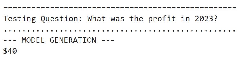
# Ask the model a question
ask_model(
    question="What was the profit in 2023?",
    pre_text=pre_text_simple,
    table=table_simple,
    post_text=post_text_simple)

The model returns the following output:

The model's answer is correct, which indicates that our fine-tuned model is working well.

• A Brief History of GPT Models

Large Language Models are immensely powerful, even in their base form. When we fine-tune them, we modify them to be tailor-made for our specific data. However, in most cases, these models are too large to be fine-tuned on consumer hardware. To overcome this challenge, we use special fine-tuning techniques called LoRAs. More specifically, the most effective way to fine-tune an LLM on consumer hardware is by using QloRA.

QLoRA represents a significant breakthrough in democratizing access to large language model fine-tuning. By combining 4-bit quantization with Low-Rank Adaptation, this technique reduces memory requirements by approximately 75% compared to traditional full fine-tuning methods. As a result, it enables fine-tuning billion-parameter models on consumer-grade GPUs.

This article covered everything you need to know about QLoRA. First, it explained the theory behind how QLoRA works. Then, it demonstrated how you can fine-tune a 7 billion parameter model on a consumer-grade GPU.