


Table of Contents
In the previous articles, I covered what emotion recognition is and how to perform emotion recognition. While modules that contain pre-built models cover a large number of use cases when it comes to detecting emotions, there are benefits to knowing how to create custom emotion recognition models.
Custom emotion recognition models can be more accurate in some situations. For example, if your company wants to introduce an emotion recognition model to gauge how people react to their ads in malls, using images of people looking at your ads to train a custom model can lead to better results than using a pre-built solution. However, even when building custom models, it is usually a better idea to leverage transfer learning in some way. This way you don't need to rely on collecting a lot of high-quality data and can get good results with smaller datasets.
In this article, I will focus on creating an emotion recognition model that can try and guess whether a person is interested in a lesson or not.
What Dataset Should You Use to Detect Emotion?
Most datasets are focused on detecting certain emotions such as happy, sad, or angry. In my case, since I just want to know whether a person is interested in a lesson or not, I don't need that kind of accuracy. For my purposes, I can split emotions into three categories: positive, neutral, and negative.
In an ideal situation, my students would display positive emotions, but even being neutral is acceptable. I am mainly trying to avoid holding classes that elicit negative emotions in my students. To train my model, I will use a modified version of the FER13 dataset, which contains 48X48 pixel images that each display a certain emotion. Because there are images that represent multiple negative emotions (such as fear and anger), I will modify my labels so that there are only three categories: positive, neutral, and negative.
Article continues below
Want to learn more? Check out some of our courses:
How to Prepare the Data for Your Model
Before I create my model, I need to prepare the data.
First, I need to import everything I will use:
# Let's import our data

import pandas as pd
import numpy as np
import tensorflow as tf
from tensorflow.keras.layers import Dense, GlobalMaxPool2D
from tensorflow.keras.models import Model
from tensorflow.keras.applications.mobilenet import MobileNet
from tensorflow.keras.optimizers import Adam
from tensorflow.keras.callbacks import ModelCheckpoint,EarlyStopping, ReduceLROnPlateau
from tensorflow.keras.preprocessing.image import ImageDataGenerator
import matplotlib.pyplot as plt
from sklearn.metrics import classification_report
I will use Keras to create my neural network and train it. When working with images in Keras, it’s best to use the ImageDataGenerator class. Using Keras ImageDataGenerator, I can take my data, augment it and load it into my model for training, and later testing.
While I can use the data augmentation techniques I plan on using for training, I shouldn’t use them for the images I plan on using for validation and testing. Therefore, I'll define separate generators for training, validation, and testing. The validation and testing generators are the same, but for the sake of clarity I will create a separate validation generator and a separate testing generator.
One thing to note: always rescale images.
Deep learning networks are very sensitive to unscaled data and will perform poorly with it.
# Define training data generator

train_datagen = ImageDataGenerator(rescale=1./255,
    shear_range=0.2,
    zoom_range=0.2,
    horizontal_flip=True)


# Define validation data and testing data generators
# Technically the same, but separated here for the
# sake of clarity

validation_datagen = ImageDataGenerator(rescale=1./255)
test_datagen = ImageDataGenerator(rescale=1./255)
This is not enough to load my data to my model. The generator itself only defines whether I want to load my data as is or if I want to change it in some way.
Essentially, it defines how I plan on loading data into my model. To specify the data source, I need to use one of the generator’s flow methods. The two most common methods are:
- flow_from_directory
- flow_from_dataframe
The more commonly used method is flow_from_directory. This method requires images to be stored in separate folders. For each class, I need to have a separate folder, and I will need to store images of that class in that directory. The generator uses the structure of my directory to assign labels to images. This may seem practical and simple at first, but it requires me to create multiple directories and can lead to extra steps. If I know how my images are labeled, there is no need to go through the process of storing them in separate directories. Instead, I can just feed labels directly to Keras.
This is where flow_from_dataframe comes into play. It allows me to store all of my images into a single directory and use a Pandas DataFrame to assign labels to them when loading them using the ImageDataGenerator class. To be more specific, I need two columns: one column with image names, and one column with labels that are associated with my images.
This skips the extra step and allows more detailed control. For example, if I want to skip some images that are in the folder, I can just remove them from the DataFrame. Also, it will be much easier to create training, validation, and testing data that way.
The first thing I will do is create a DataFrame from my CSV file.
# Read in data into a DataFrame

df = pd.read_csv("image_dataset.csv")
This DataFrame consists of two columns: "files" and "target." The "files" column represents my images, while the "target" column represents image labels.
Now that the DataFrame has been loaded, I'll modify the labels a bit. As I mentioned earlier, I am not interested in specific emotions, just in whether they are positive, negative, or neutral. Because I will use the flow_from_dataframe method, I need to make sure that my labels are properly defined, so I'll map negative emotions to the "negative" label, positive to the "positive" label, and neutral to the "neutral" label.
# Map values to positive, negative, neutral

mapping = {"Anger":"Negative",
           "Happiness":"Positive",
           "Fear":"Negative",
           "Neutral":"Neutral"}

df["target"] = df["target"].map(mapping)
Now that the labels have been re-mapped, let's shuffle our dataset and separate my data into training, validation, and testing data.
# Shuffle data

df = df.sample(frac=1).reset_index(drop=True)

# Separate data into training, validation, and test data

train = int(len(df)*0.75)
test = int(len(df)*0.9)

df_train = df.iloc[:train, :].copy()
df_validation = df.iloc[train:test, :].copy()
df_test = df.iloc[test:, :].copy()
Now both my ImageDataGenerator class and my three DataFrames are prepared.
Let's use the flow_from_dataframe method to define how I will access my data:
# Get training data

train_data = train_datagen.flow_from_dataframe(
    dataframe=df_train,
    target_size=(128,128),
    batch_size=32,
    directory="data",
    x_col="files",
    y_col="target")

# Get validation data

validation_data = validation_datagen.flow_from_dataframe(
    dataframe=df_validation,
    target_size=(128,128),
    batch_size=32,
    directory="data",
    x_col="files",
    y_col="target")

# Get testing data

test_data = test_datagen.flow_from_dataframe(
    dataframe=df_test,
    target_size=(128,128),
    batch_size=32,
    shuffle=False,
    directory="data",
    x_col="files",
    y_col="target")
There are two important things to note here:
First, my images are 48x48 pixels in size, while the smallest dimension of the images the MobileNet network was trained on is 128x128. Since I plan on using pretrained weights, I will scale my images to 128x128. Upscaling somewhat decreases the quality of my images, but it is a necessary sacrifice.
Second, in test_data it is of extreme importance that I strictly define the parameter shuffle as False. Otherwise, I won't be able to test the performance of my model.
How to Create a Custom Model
The model I will use for emotion recognition is a model built on top of the MobileNet network. To be specific, I will use a version of MobileNet pretrained on the imagenet dataset. However, I won't include the top of the MobileNet model. Instead, I will add a global max-pooling layer and a dense prediction layer on top of it.
To finish, I will freeze the first 15 layers of the model:
#Create model

mobile_net = MobileNet(
    input_shape=(128, 128, 3),
    include_top=False,
    weights="imagenet",
    classes=3
)
mobile_net_output = mobile_net.layers[-14].output
global_pool = GlobalMaxPool2D(name="global_pool")(mobile_net_output)
out = Dense(3, activation="softmax", name="out_layer")(global_pool)
model = Model(inputs=mobile_net.input, outputs=out)

for layer in model.layers[:15]:
    layer.trainable = False
Now that I've defined my custom model, it is time to compile it. The loss function I will use is categorical cross-entropy. I will use Adam as my optimizer and I will track accuracy.
# Compile model

model.compile(loss="categorical_crossentropy", optimizer=Adam(0.01), metrics=["accuracy"])
Before running our model, I will also define some callbacks:
- ModelCheckpoint - to checkpoint our data and save results
- EarlyStopping - to stop the model if it doesn't improve for a certain number of epochs
- ReduceLROnPlateau - to reduce the learning rate if the model stops learning
# Define a path where we want to save the model

filepath = "models"

# Define some callbacks

checkpoint = ModelCheckpoint(
    filepath,
    monitor="val_accuracy",
    verbose=1,
    save_best_only=True,
    mode="max")

earlystopping = EarlyStopping(
    monitor="val_accuracy",
    patience=15,
    verbose=1,
    mode="auto",
    restore_best_weights=True)

rlrop = ReduceLROnPlateau(
    monitor="val_accuracy",
    mode="max",
    patience=5,
    factor=0.5,
    min_lr=1e-6,
    verbose=1)

# Create a list of callbacks

callbacks = [checkpoint, earlystopping, rlrop]
How to Train the Model
Now that everything is ready, I can go ahead and train my model:
# Train the model
history = model.fit(
train_data,
validation_data=validation_data,
epochs=25,
steps_per_epoch=len(train_data),
validation_steps=len(validation_data),
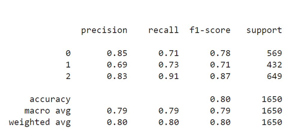
callbacks=callbacks)Classification accuracy by itself can be misleading.
Therefore, it is a much better idea to take a look at a classification report instead:
# Get predictions

predictions = np.argmax(model.predict(test_data), axis=-1)


# Get the classification report

print(classification_report(test_data.classes, predictions))
The result I get by running this code is:
Image Source: Screenshot, Edlitera
The problem I currently faced with is that I don't know which of the three labels represents which class.
To access that data, I can simply access the class_indices attribute of my generator object.
# Get dictionary that connects labels with their integer representations

labels = (train_data.class_indices)
labels
The result I get by running this code is a dictionary that connects classes with their integer representations:
{'Negative': 0, 'Neutral': 1, 'Positive': 2}Finally, let's visualize the results:
# Show training history

def visualize_train_history(train_history,train,test):
    plt.plot(train_history.history[train])
    plt.plot(train_history.history[test])
    plt.title("Training History")
    plt.ylabel(train)
    plt.xlabel("Epoch")
    plt.legend(["Train", "Test"], loc="upper left")
    plt.show()

visualize_train_history(history, "loss", "val_loss")
visualize_train_history(history, "accuracy", "val_accuracy")
What is Super-resolution as a Data Preprocessing Technique?
I used some basic data preprocessing in the form of simple image augmentations implemented by the Keras ImageDataGenerator. While this allowed me to achieve a good baseline accuracy, let's see if I can get even better results by using more advanced techniques.
One of the fields of computer vision that has gained quite a lot of traction in recent times is super-resolution. Super-resolution imaging is a technique that consists of increasing the resolution of images. This technique was developed to solve one very simple but frequent issue, which is that training set images are often smaller resolution than commonly used models expect. Using super-resolution can therefore be considered a non-typical image augmentation technique.
This doesn't mean you should avoid using typical image augmentation techniques, some of which are:
- Rotation
- Translation
- Color Augmentations
- Flipping
- Cropping
- Adding noise
- Blurring
I won't focus on these techniques in this article because they serve a different purpose to compensate for data loss by increasing the size of your dataset. Using standard image augmentation techniques will increase the number of different images our model trains on. That increase in size is usually enough to improve the accuracy of your models.
In this article, I focus on trying to improve accuracy without actually increasing the size of your training dataset, but instead by introducing modern data upscaling techniques. The size of your dataset will stay the same, but the resolution of the images inside it will be bigger. This is also why I won't add any new data augmentation techniques aside from increasing the resolution of my images. If I used additional augmentation methods (aside from those I used earlier on in this article) it would be very hard to gauge whether using super-resolution helped my model achieve higher accuracy or whether it was the consequence of using those other image augmentation techniques.
To increase the resolution of my images I will use special neural networks designed for upscaling images while minimizing data loss. I don't even need to create such a network myself. Fortunately, it is very easy to implement such a network using OpenCV.
Let's import everything I need to upscale my images:
# Import necessary libraries

import cv2
import os
Then I need to define the Super Resolution object:
# Create a SR object

sr = cv2.dnn_superres.DnnSuperResImpl_create()
Since I am using a pre-trained model to upscale my images, I need to download the trained model and point Python to it:
# Define path to SR model

path_to_model = "EDSR_x4.pb"
Now everything is ready. I can read in the model that I defined:
# Read the model

sr.readModel(path_to_model)
sr.setModel("edsr",4)
The second parameter I define while setting the model tells Python how much I want to upscale my images. My goal here is to upscale an image so that it matches one of the image sizes that MobileNet was originally trained on.
I have chosen 4, which means that the dimensions of my image will be 4 times bigger. This leads to an image size of 192x192. This will allow me to feed 192x192 images into my network without needing to upscale them using Keras ImageDataGenerator.
Since all of my original images are stored in the data directory, I will create a new one and call it processed_data. Each image in my data directory will get upscaled and stored inside the newly-created directory:
# Define paths to original directory and new directory

new_directory_path = "processed_data"
original_directory_path = "data"

# List images in the original directory

list_of_images = os.listdir(original_directory_path)

# Upscale images and store them in the new directory

for image_name in list_of_images:
    image = cv2.imread(f"{original_directory_path}/{image_name}")
    result = sr.upsample(image)
    cv2.imwrite(f"{new_directory_path}/{image_name}", result)
To re-run my code from earlier and use these upscaled, higher resolution images, I need to somewhat modify my code. I need to change the parts of our code that reference the size of our images.
Those parts are:
# Get training data
train_data = train_datagen.flow_from_dataframe(
dataframe=df_train,
target_size=(192,192),
batch_size=32,
directory="processed_data",
x_col="files",
y_col="target")
# Get validation data
validation_data = validation_datagen.flow_from_dataframe(
dataframe=df_validation,
target_size=(192,192),
batch_size=32,
directory="processed_data",
x_col="files",
y_col="target")
# Get testing data
test_data = test_datagen.flow_from_dataframe(
dataframe=df_test,
target_size=(192,192),
batch_size=32,
shuffle=False,
directory="processed_data",
x_col="files",
y_col="target")
# Define model
mobile_net = MobileNet(
input_shape = (192, 192, 3),
include_top = False,
weights = "imagenet",
classes = 3)
x = mobile_net.layers[-14].output
global_pool = GlobalMaxPool2D(name="global_pool")(x)
out = Dense(3, activation="softmax", name="out_layer")(global_pool)
model = Model(inputs=mobile_net.input, outputs=out)
for layer in model.layers[:15]:
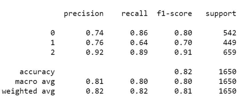
layer.trainable = FalseOnce I retrain the network, I get the following results:
Source Image: Screenshot, Edlitera
My results are noticeably better. The change from 0.8 to 0.82 might not seem like much, but it is actually quite big if you take into consideration that this is just one technique and that the increase in accuracy I get from it can't be compared to using sets of augmentations.
When you see bigger increases in accuracy in other examples, they are the product of using a set of augmentations, which in implementation look somewhat like this:
train_datagen = ImageDataGenerator(
    rescale=1./255,
    shear_range=0.2,
    zoom_range=0.2,
    width_shift_range=0.25,
    height_shift_range=0.25,
    rotation_range=10,
    brightness_range=[0.2, 1.2],
    horizontal_flip=True)
Such a set would probably lead to better results, but as you can see it is actually a combination of more than 5 different augmentation techniques.
Combining the results I got by upscaling my data from 48x48 to 192x192 with a set of augmentations such as the one I just defined is actually what would lead to the best possible results. So when designing and training a neural network, you should not limit yourself to the most common practices, but should also try to use your knowledge from other fields to improve your results.
In this article, I demonstrated that it is possible to build a model that would gauge how interested students are in a particular lecture. By tracking whether students exhibit positive, neutral, or negative emotions during a lecture, an instructor could track which parts of the lecture are interesting and which parts may still require some adjustments to better captivate students. Great results were achieved on a fairly limited dataset, which means that there is potential for even better results with a better dataset. This is especially true when you consider that the results I got represent what can be achieved without too much model tuning, and while using almost no traditional data augmentation techniques.
Since I didn't opt for traditional data augmentation techniques, I decided to implement something else: upscaling using neural networks. This idea led to a noticeably better result and should be considered alongside implementing traditional image augmentation techniques (such as rotation, translation, color augmentation, zooming, flipping, or cropping) if you want to try and achieve the best possible results with the model presented in this article.
Overall, this series of articles was designed to demonstrate the importance of emotion AI and emotion recognition, and how you can implement and use emotion recognition. The previous article in the series was designed to give readers an easy way of performing emotion recognition with just a few lines of code, while this one delved deeper into what you need to do to train your model and showed that there is a potential application of this technology in the education industry.

