


Table of Contents
Pandas is the premier library for data manipulation and analysis in Python. It is the preferred tool for handling all types of data, including time series data. In a previous article in this series, I discussed the datetime library. Now I’ll demonstrate how Pandas builds around the datetime library to allow you to efficiently work with time series data.
- Previous article: How to Handle Time Series Data Sets
- Intro to Programming: What Are Packages in Python?
- Intro to Pandas: What is Pandas in Python?
In this article, I will show you how easy it is to perform some of the most important operations in time series analysis using Pandas, such as indexing, slicing, and resampling.
How to Use the DatetimeIndex in Pandas
To demonstrate how you handle time series data, I will use the Power Consumption dataset from Tetouan City, made available by the UCI Machine Learning Repository. In the dataset you will find the energy consumption of this North-Moroccan city in 10 minute intervals. It comes with a DateTime column that I will need to parse before moving on to more complex operations.
Of course, before doing anything else, I need to import the Pandas library:
# Import the Pandas module
import pandas as pd
After importing the Pandas library, it is time to load the data.
I can load the data set directly from the UCI repository using the read_csv() method of Pandas:
# Load the data
url = 'https://archive.ics.uci.edu/ml/machine-learning-databases/00616/Tetuan%20City%20power%20consumption.csv'
df = pd.read_csv(url)
After loading the data, I can take an initial look at it by displaying the first five rows using the head() method:
# Display the first five rows of the DataFrame
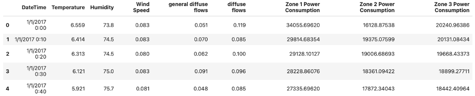
df.head()The result I get by running the code above is:
A DataFrame of the Power Consumption dataset of Tetouan City.
Image Source: Edlitera
Immediately, you notice that the index is a simple RangeIndex and not a DatetimeIndex. However, I have a column that contains data about the year, month, day and time, called DateTime. When dealing with time series data, you always want to make sure that this data is contained in the index and not in one of the columns, so you need to replace the index with the data stored inside the DateTime column.
- Intro to Pandas: How to Analyze Pandas DataFrames
- Intro to Pandas: What is a Pandas DataFrame and How to Create One
However, before I do that, I want to demonstrate that you should always check the data type of each column, because numeric or time data can often be in the form of strings, which you do not want.
So, to check the type of data in my columns, I can use the info() method from Pandas:
# Inspect data types
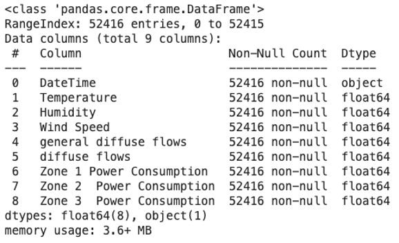
data.info()I get the following result by running the code above:
Checking the data provided by the Power Consumption dataset of Tetouan City in each column using the info() method from Pandas.
Image Source: Edlitera
It seems that the data in my DateTime column is in fact stored in a string, as shown by the fact that its dtype above is object. Fortunately, Pandas offers a simple parsing solution: pandas.to_datetime(). This top-level function converts a column from various formats to datetime. In most cases, it automatically works out the correct formatting.
So I’ll use it to transform my data from one data type to another. I will also check whether the conversion was successful:
# Cast the DateTime column to datetime format
df['DateTime'] = pd.to_datetime(df['DateTime'])
# Inspect data types
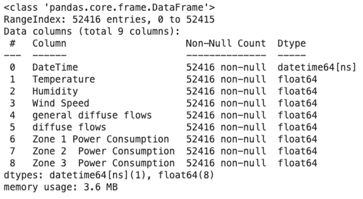
df.info()The result I get after running the code above is as follows:
The Power Consumption dataset of Tetouan City converted from string data type into DateTime data type.
Image Source: Edlitera
As you can see in the image above, the dtype of the DateTime column is now datetime, so I have successfully converted my data.
When using this method, there are two important parameters that I did not use here, because they often lead to problems:
- The errors parameter
- The infer_datetime_format parameter
The errors parameter allows you to ignore entries that the function could not parse, instead of raising an error and invalidating the entire process. Using this parameter is not recommended because it essentially hides errors that Pandas runs into while completing the operation. Instead, you'd probably agreed that it is much better to know about problematic data, so you can either fix it or get rid of it.
The infer_datetime_format parameter can significantly speed up the parsing process. It works out the datetime format from the first element of the input and uses it for every other entry. It often speeds up the process by five to ten times, but it can be risky to use. In some situations, your data may be formatted differently in different rows, so if you tell Pandas to always parse data as if it was formatted in the same way as the data in the first row, you could run into some problems.
Now that the data in the DateTime column is ready, I can set it as the index of my data using the set_index() method of Pandas.
I’ll also use the head() method to display the result:
# Set DateTime as the index of our DataFrame
df.set_index('DateTime', inplace=True)
# Display the first five rows of our DataFrame
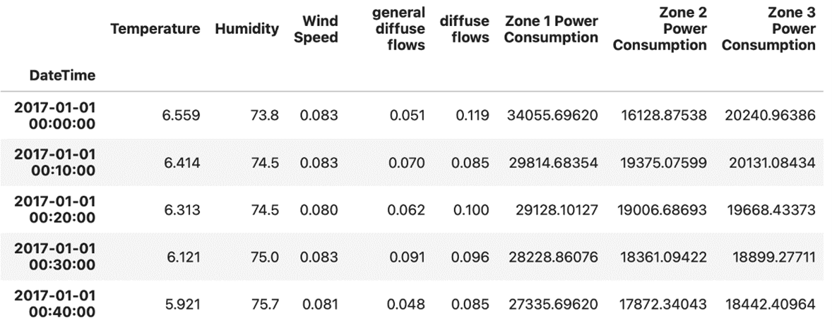
df.head()The first five rows of the DataFrame I get by running the code above look like this:
The Power Consumption dataset of Tetouan City showing the first five rows set to DateTime as the index in the DataFrame.
Image Source: Edlitera
If I check the type of index I currently have, I’ll see that it is a DatetimeIndex.
Article continues below
Want to learn more? Check out some of our courses:
How to Filter Data with the DatetimeIndex in Pandas
The DatetimeIndex is a specialized type of index that allows you to convert time series data into an index. It can perform a lot of different functions that help you efficiently analyze your time series data.
The most basic thing you can do is to extract every fraction of the datetime information. From this point onward, understanding how the datetime module works is very important, so if you are not familiar with it, I highly suggest going over the previous article in this series, because it covers in-depth how you use the datetime module.
I’ll first import what I need from the datetime module:
# Import the date and time classes
from datetime import date, time
Next, I’ll extract rows where the time in my DatetimeIndex is 12:10 AM:
# Filter data
mask = df.index.time==time(12,10)
df[mask]
The result I get by running the code above is:
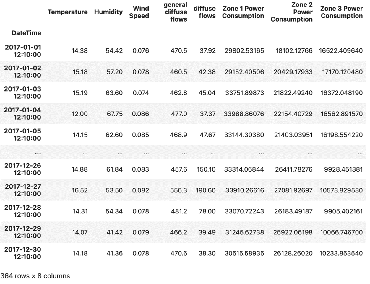
Extracted DataFrame rows from the Power Consumption dataset of Tetouan City with time in the DatetimeIndex is set to 12:10 A.M using Pandas.
Image Source: Edlitera
I can also filter my data to get information on a particular date:
# Filter to get all data we have for the date 2017-05-05
mask= df.index.date==date(2017,5,5)
df[mask]
The result I get by running the code above is:
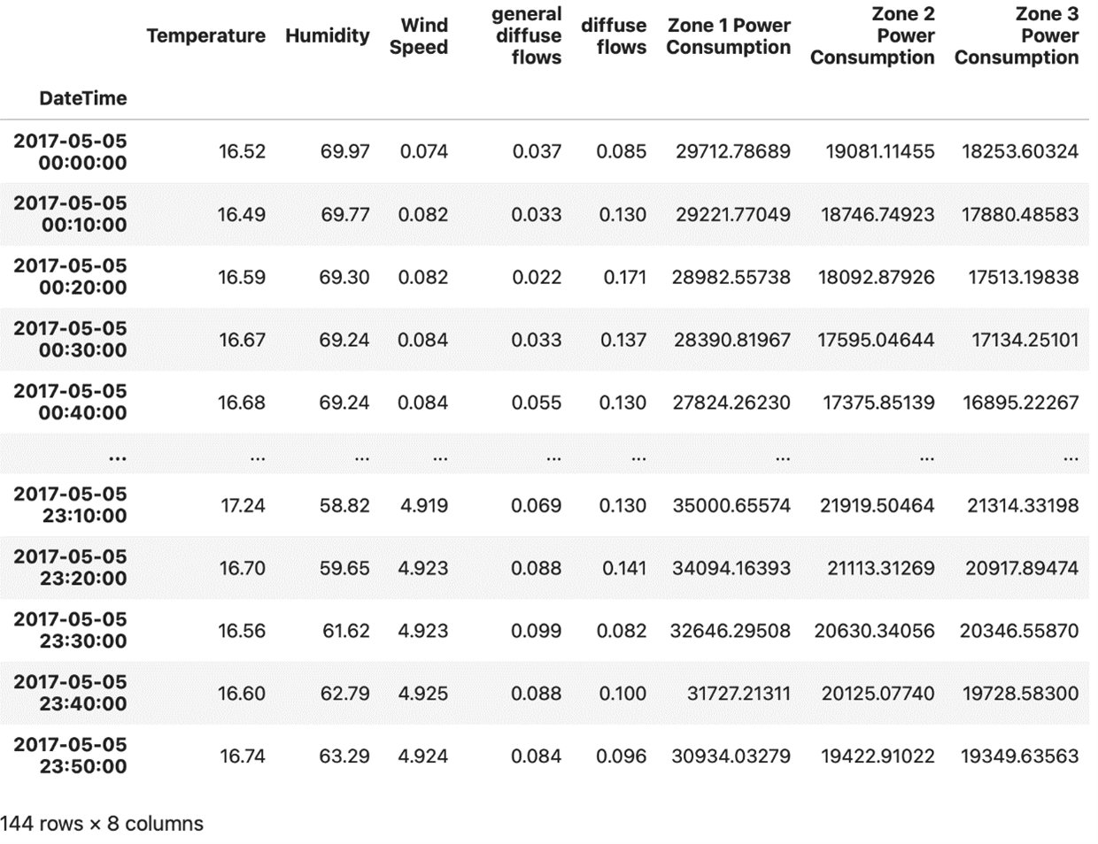
A DataFrame of the Power Consumption dataset of Tetouan City filtered to show a specific date using Pandas.
Image Source: Edlitera
I can be even more precise. I’ll filter my DataFrame so that I get information on the different values of my features at noon every Monday:
# Filter to get data about values
# for noon of every Monday
mask = (df.index.weekday==1) & (df.index.time==time(12,0))
df[mask]
The result I get by running the code above is:
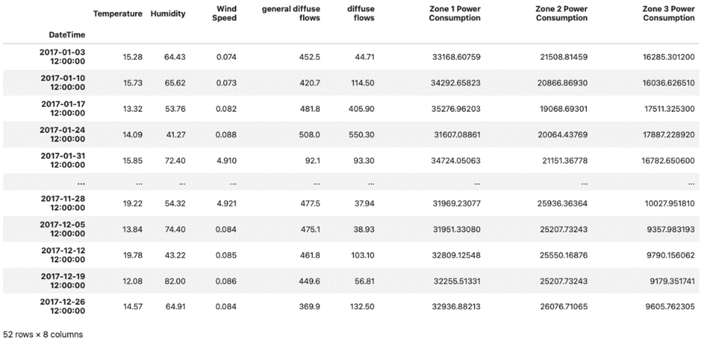
A DataFrame of the Power Consumption dataset of Tetouan City filtered to show the different values of features for “noon every Monday.”
Image Source: Edlitera
While everything demonstrated above is useful in and of itself, the true power of filtering data like this becomes apparent when you start analyzing each feature separately. Let's say that I want to learn more about power consumption in Zone 1. For example, what was the power consumption in Zone 1 on May 5th of 2017?
What I can do is separate the Zone 1 data as a Pandas series and then filter out the day I'm interested in:
# Restrict the data to Zone 1 Power Consumption
zone1 = df['Zone 1 Power Consumption']

# Filter out data for May 5th of 2017
mask = df.index.date==date(2017,5,5)
power_consumption = zone1[mask]
power_consumption
The result I get by running the code above is:
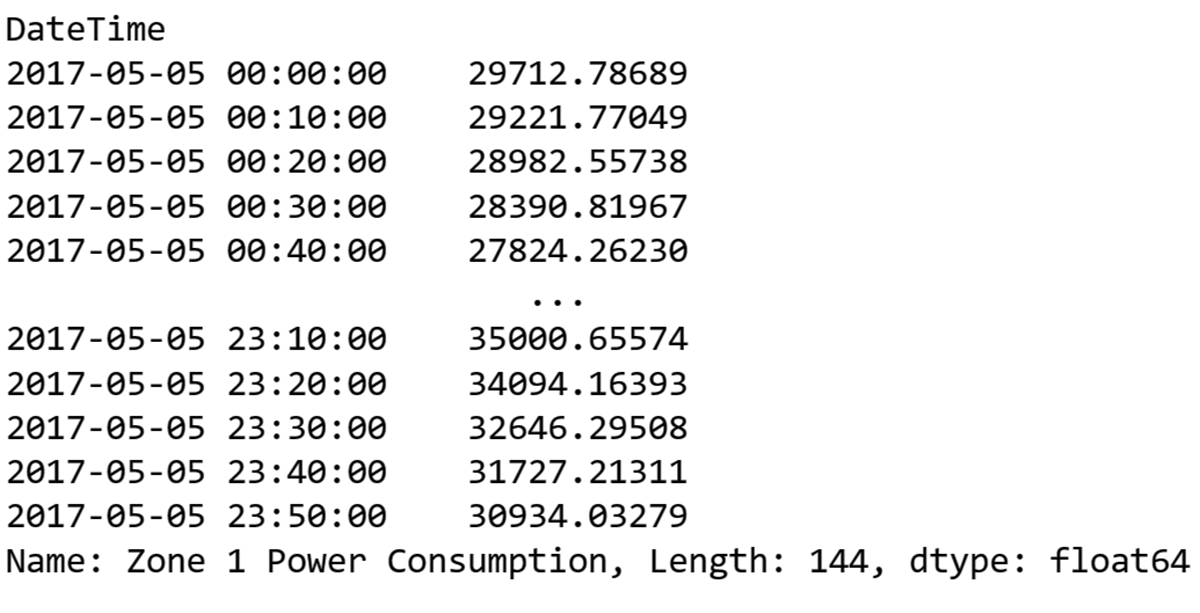
Filtered out data to show the power consumption of Zone 1 from the Power Consumption dataset of Tetouan City using Pandas time series.
Image Source: Edlitera
The results are even more impressive if you also create visualizations. I won't focus on those in this article, but just to demonstrate, I’ll create a line plot to visualize the data from my latest filter operation:
# Import the library we will use to create visualizations
import matplotlib.pyplot as plt

# Create a line plot of filtered data
power_consumption.plot(
	figsize=(14,5),
	title='Power Consumption 2017/05/05')
The result I get by running the code above is:
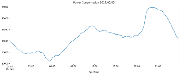
A line plot to visualize the filtered data from Power Consumption dataset of Tetouan City showing Zone 1’s power consumption on 05-05-2017.
Image Source: Edlitera
The plot above shows consumption peaks at 12:00 and 21:00. For example, the pick at 21:00 might indicate that Zone 1 is a residential one, where an increase of energy would be expected outside of working hours because those are times many people use power to cook lunch or watch TV in the evening.
Even though filtering is a powerful way to analyze data, you also need other tools to fully understand what your data is telling you. This is easy to see if, instead of filtering for a specific day, I want to, for example, display and plot power consumption in Zone 1 for each day at 12:10 AM:
# Filter out data for 12:10 AM
mask = df.index.time==time(12,10)
power_consumption_12_10 = zone1[mask]

# Plot the Zone 1 Power Consumption daily at 12:10 AM
power_consumption_12_10.plot(
	figsize=(14,5),
	title='Power Consumption at 12:10 AM')
The result I get by running the code above is:
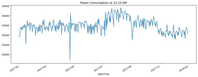
A line plot to visualize the filtered data from Power Consumption dataset of Tetouan City showing Zone 1’s power consumption every day at 12:10 A.M.
Image Source: Edlitera
There is clearly one extreme fall in power consumption, but how can you determine exactly when it is by looking at the graph? The best way to solve a problem like this it to slice the DatetimeIndex.
How to Use Slicing with the DatetimeIndex in Pandas
Apart from filtering, slicing is an essential tool that can significantly simplify and streamline your analysis. It allows you to effortlessly select and manipulate subsets of data.
To slice the DatetimeIndex you just need to input a certain date range in ISO format to the loc indexer. Let's look at how I would slice my example Power Consumption DataFrame so that I get just the power consumption in Zone 1 for the second half of April.
Note that the slice will include both the starting and end dates:
# Slice of dt corresponding to the second half of April
zone1.loc[‘2017-04-15’:’2017-04-30’]
The result I get by running the code above is:
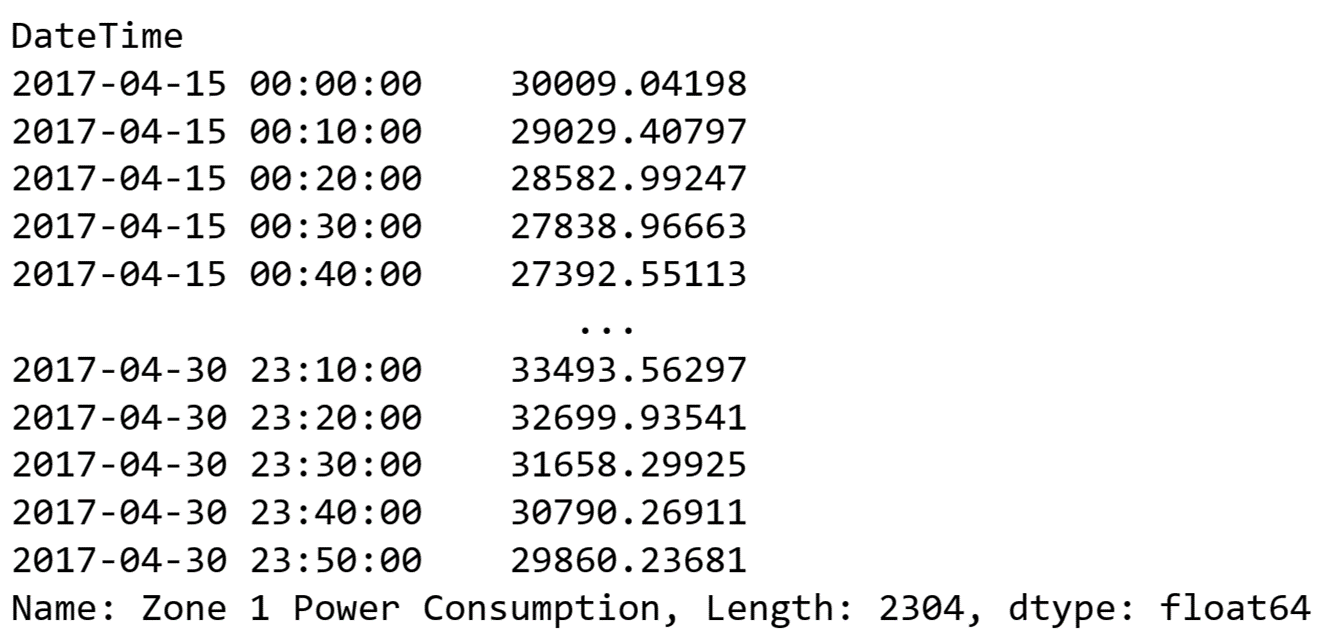
Sliced data from the Power Consumption dataset of Tetouan City showing the power consumption of Zone 1 for the second half of April in 2017.
Image Source: Edlitera
This way of slicing is possible because of the DatetimeIndex. It allows you to use any string that can be converted to a timestamp to slice your data. Of course, you can be even more precise and add hours to slices. What's even more impressive is that you can define your slice so that it returns data from multiple columns by slicing the DataFrame itself instead of a Pandas series that represents just one column of data.
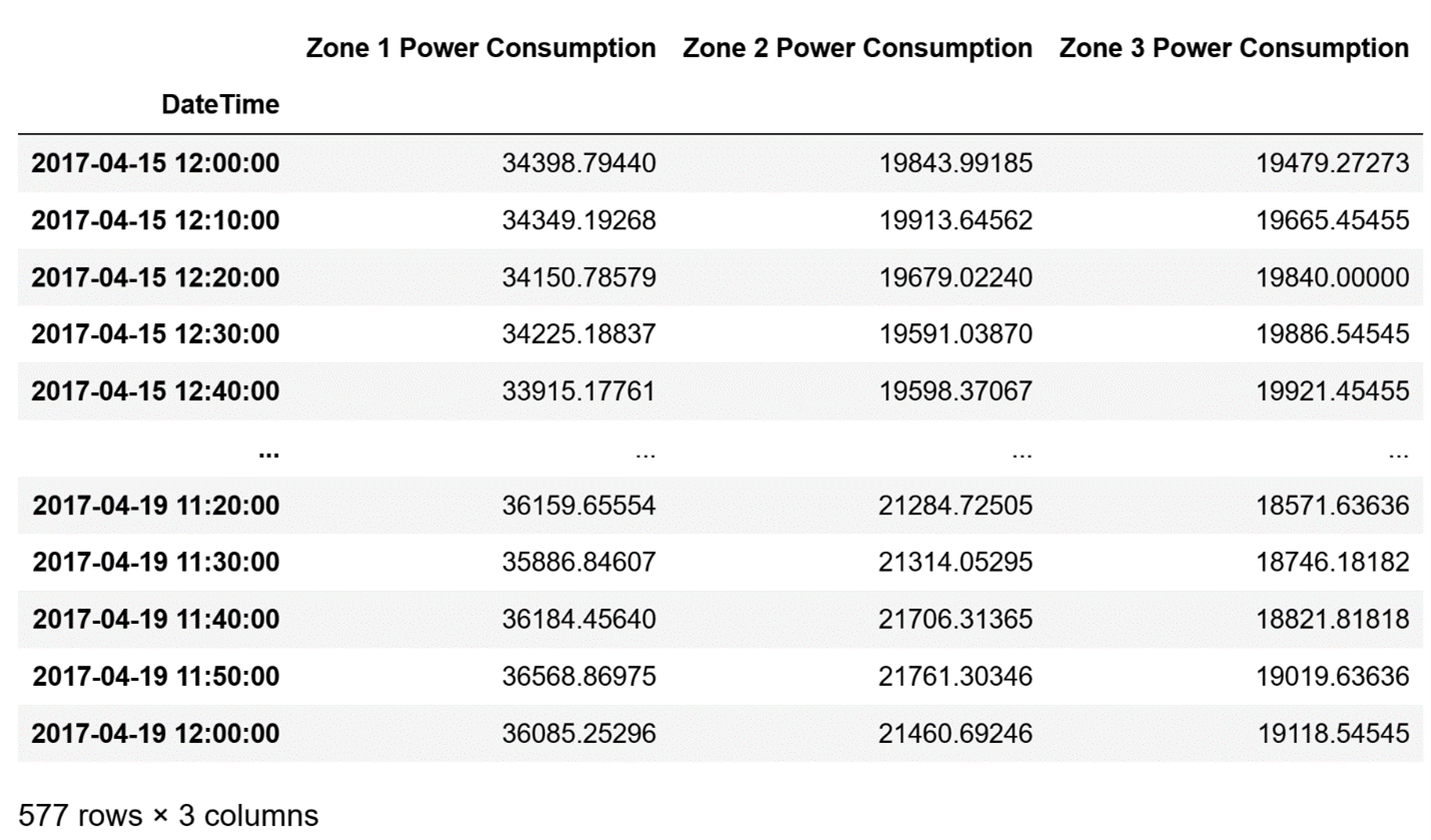
I'll return data about the power consumption from all zones starting at noon on the 15th of April and ending at noon on the 19th of April:
# Define columns of interest
columns_of_interest = [
	'Zone 1 Power Consumption',
	'Zone 2 Power Consumption',
	'Zone 3 Power Consumption'
]

# Slice df to return wanted data
df.loc['2017-04-15 12:00':'2017-04-19 12:00', columns_of_interest]
The result I get by running the code above is:
A slice of the DatetimeIndex from the Power Consumption dataset of Tetouan City showing all zones’ power consumption from the 15th of April to the 19th of April.
Image Source: Edlitera
How to Sort a DataFrame with the DatetimeIndex in Pandas
Sorting a DataFrame with DatetimeIndex is simple with the sort_index() method. To demonstrate how it works, I’ll shuffle my DataFrame to make it messy on purpose, and then use the sort_index() method to sort my data:
# Shuffle our DataFrame
shuffled_df = df.sample(frac=1)
The result I get by running the code above is the following shuffled version of my DataFrame:
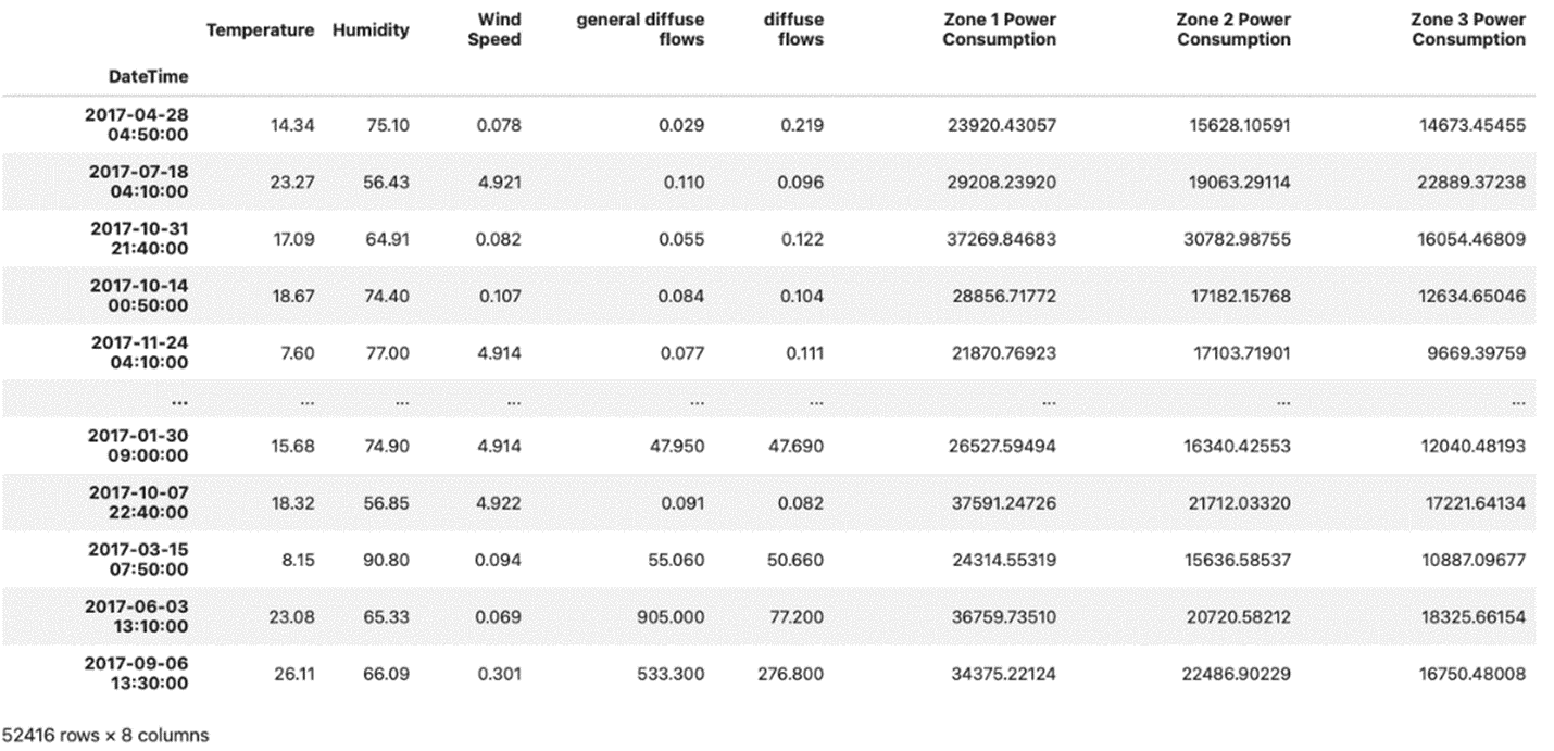
A DataFrame with shuffled data from the Power Consumption data set of Tetouan City.
Image Source: Edlitera
Sometimes, you will get datasets such as the one in the image above. In that case, when you are working with time series data, the first thing to do is to sort your data. You can sort it in ascending or descending order.
I’ll first demonstrate sorting it in ascending order:
# Sort the DataFrame by the DatetimeIndex in ascending order
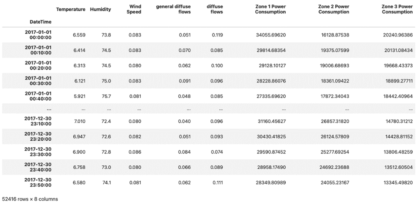
shuffled_df.sort_index()The result I get by running the code above is the following sorted version of my DataFrame:
DataFrame with data sorted in ascending order.
Image Source: Edlitera
As you can see, the data above is sorted in ascending order. To sort in descending order, you need to set the value of the ascending argument of the sort_index() function to False:
# Sort the DataFrame by the DatetimeIndex in descending order
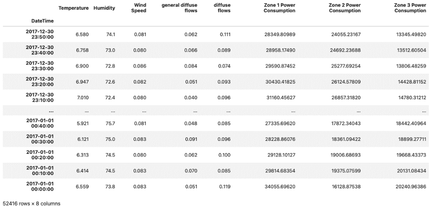
shuffled_df.sort_index(ascending=False)The result I get by running the code above is the following sorted version of my DataFrame:
DataFrame with data sorted in descending order.
Image Source: Edlitera
Pandas is one of the most powerful and flexible tools in Python for data analysis, and as such, it should come as no surprise that it is also very popular for analyzing time series data. Many data analysts choose Pandas for time series analysis because it provides easy ways of manipulating the data. For example, the DatetimeIndex makes performing most operations in Pandas very simple, as it allows you to index, slice, and resample data based on the date and time. Another popular feature of Pandas is the straightforward graph plotting using the DatetimeIndex. These and other features make it easy to understand why Pandas is considered the best tool for time series data analysis in Python.

