

![[Future of Work Ep. 1] Future of Fashion: Using Data to Predict What Will Sell with Julie Evans](https://res.cloudinary.com/edlitera/image/upload/ar_16:9,c_fill,f_auto,q_auto,w_100/56ar4tdmijwmrgnhoq4f56kcoddw?_a=BACJ3SGT)
Table of Contents
- What is the Decoder Block?
- How to Use the Positional Encoder
- How to Use the Masked Multi-Head Self-Attention Layer
- How to Use the Encoder-Decoder Attention Layer
- How to Use the Feed-Forward Network and the Final Linear Layer
- How Does the Transformer Model Perform Translation
- What Are the Differences Between the Original Transformer Model and GPT?
In the first part of this series about Transformers, I explained the motivation for creating the Transformer architecture and how one of its main parts, the Encoder, works. In this article, I will wrap up my explanation of the Transformer architecture by explaining what happens in the Decoder block. The structure of the Decoder block is similar to the structure of the Encoder block, but it has some minor differences. To explain these differences, I’ll continue with the example of translating text from one language to another, which is the task the Transformer model originally designed for.
- Previous article: Intro to Transformers: The Encoder Block
What is the Decoder Block?
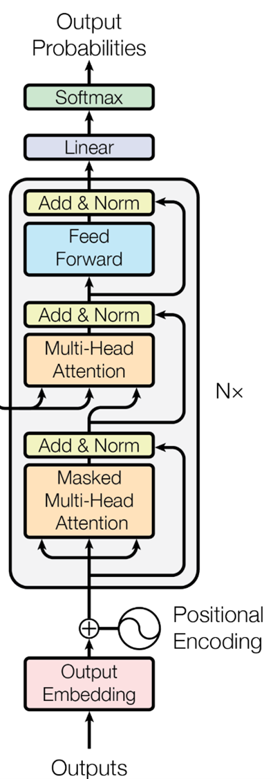
The Decoder block
Image Source: Vaswani, A., et al. "Attention is all you need." Advances in neural information processing systems 30 (2017).
The Decoder block is an essential component of the Transformer model that generates output sequences by interpreting encoded input sequences processed by the Encoder block. It is composed of five distinct parts:
- Positional Encoder
- Masked Multi-Head Self-Attention Layer
- Encoder-Decoder Attention Layer
- Feed-Forward network
- Final Linear layer
How to Use the Positional Encoder
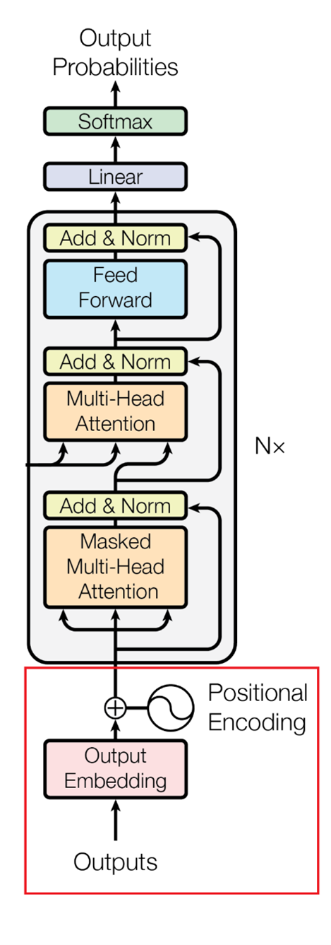
The Positional Encoder
Image Source: Vaswani, A., et al. "Attention is all you need." Advances in neural information processing systems 30 (2017).
The Positional Encoder in the Decoder block operates similarly to its counterpart in the Encoder block, encoding the target language sentence instead. For instance, let’s consider translating this English sentence, "The dog barked at the cat," into French, which is "Le chien a aboyé au chat." I must first positionally encode the French sentence, just like I did with the English sentence in part one.
Assuming 4-dimensional word vectors for the translated sentence, it will look like this:
- Le: [0.25, 0.35, 0.42, 0.50]
- chien: [0.60, 0.70, 0.80, 0.90]
- a: [1.05, 1.15, 1.20, 1.25]
- aboyé: [1.40, 1.50, 1.60, 1.70]
- au: [1.85, 1.95, 2.00, 2.10]
- chat: [2.15, 2.25, 2.35, 2.45]
The Positional Encoder integrates positional data into the word vectors by creating positional vectors, which are generated using the same technique as the Encoder block uses:
- Position 1: [0.01, 0.02, 0.03, 0.04]
- Position 2: [0.05, 0.06, 0.07, 0.08]
- Position 3: [0.09, 0.10, 0.11, 0.12]
- Position 4: [0.13, 0.14, 0.15, 0.16]
- Position 5: [0.17, 0.18, 0.19, 0.20]
- Position 6: [0.21, 0.22, 0.23, 0.24]
To obtain positionally encoded word vectors for the French sentence, you do the same thing I did in the Encoder block; you sum the word vectors and their corresponding positional vectors:
- Le (position 1): [0.25+0.01, 0.35+0.02, 0.42+0.03, 0.50+0.04] = [0.26, 0.37, 0.45, 0.54]
- chien (position 2): [0.60+0.05, 0.70+0.06, 0.80+0.07, 0.90+0.08] = [0.65, 0.76, 0.87, 0.98]
- a (position 3): [1.05+0.09, 1.15+0.10, 1.20+0.11, 1.25+0.12] = [1.14, 1.25, 1.31, 1.37]
- aboyé (position 4): [1.40+0.13, 1.50+0.14, 1.60+0.15, 1.70+0.16] = [1.53, 1.64, 1.75, 1.86]
- au (position 5): [1.85+0.17, 1.95+0.18, 2.00+0.19, 2.10+0.20] = [2.02, 2.13, 2.19, 2.30]
- chat (position 6): [2.15+0.21, 2.25+0.22, 2.35+0.23, 2.45+0.24] = [2.36, 2.47, 2.58,2.69]
With the word vectors now containing positional information, you can feed them into the next part of the Decoder block.
Article continues below
Want to learn more? Check out some of our courses:
How to Use the Masked Multi-Head Self-Attention Layer
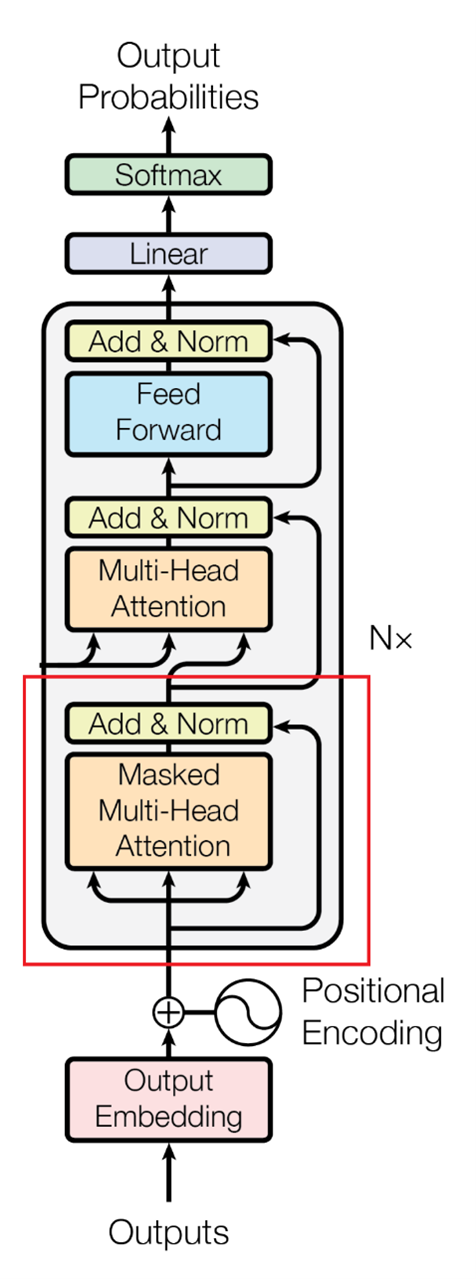
Image Source: Vaswani, A., et al. "Attention is all you need." Advances in neural information processing systems 30 (2017).
The Masked Multi-Head Self-Attention component in the Decoder block resembles the Multi-Head Self-Attention in the Encoder, but there is one crucial distinction: a "mask" is employed to prevent the model from considering words following the target word in the sentence.
For instance, consider the word "aboyé" in the French sentence of my example. A Standard Multi-Head Self-Attention layer would examine all words in the sentence and calculate their importance to the target word. However, a Masked Multi-Head Self-Attention layer only considers words preceding the target word and deems the following words irrelevant.
Mathematically, the Masked Multi-Head Self-Attention layer calculates word vectors for each word before and after your target word (in this case, "aboyé"), but sets the attention vectors for words after the target word to negative infinity. This is because attention scores are passed through a Softmax function after being calculated to obtain probabilities, as in the Encoder block. Setting the masked word’s attention scores to negative infinity results in a probability value of zero, rendering the model's perceived importance of these words to the target word negligible. The weighted sum of word vectors is computed using the normalized attention scores, and this process is repeated for each word in the sentence multiple times (once per attention head).
The outputs from each attention head are concatenated, resulting in a final output vector for each word in the sentence. The exact process of calculating these attention vectors is very complex, so I won't go into it in detail here.
For our purposes, these are the approximate values of the vectors that you end up with:
- Le: [0.26, 0.37, 0.45, 0.54]
- chien: [0.49, 0.60, 0.72, 0.83]
- a: [0.83, 0.95, 1.04, 1.14]
- aboyé: [0.91, 1.02, 1.14, 1.25]
- au: [1.42, 1.53, 1.64, 1.75]
- chat: [1.75, 1.86, 1.98, 2.09]
How to Use the Encoder-Decoder Attention Layer
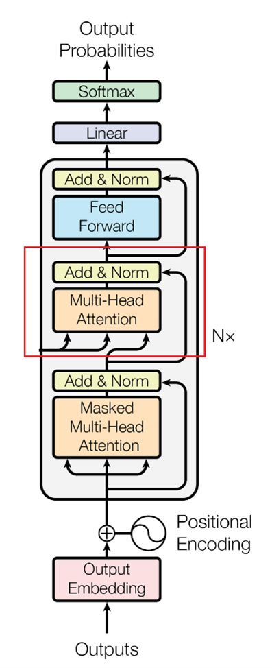
Image Source: Vaswani, A., et al. "Attention is all you need." Advances in neural information processing systems 30 (2017).
The Encoder-Decoder Attention layer enables the Decoder to concentrate on relevant portions of the input sequence while generating an output. It considers the interaction between words from the Encoder block and the words computed in the previous part of the Decoder block. I’ll break down the Encoder-Decoder Attention block into multiple steps. To simplify, I'll demonstrate this with the first target word, "Le," but the same steps apply to all other words.
The first thing you will need to do is calculate the compatibility scores. To compute compatibility scores between "Le" and each word in the English source sentence, you will use a similarity measure. In my example, I calculated the dot product between word vectors, but you can also use other similarity measures:
- Le_dot_The = [0.52, 0.94, 1.05, 0.67] . [0.48, 0.92, 1.03, 0.65] = 2.4012
- Le_dot_dog = [0.52, 0.94, 1.05, 0.67] . [1.01, 1.10, 1.21, 1.32] = 3.7601
- Le_dot_barked = [0.52, 0.94, 1.05, 0.67] . [1.35, 1.57, 1.68, 1.73] = 4.7624
- Le_dot_at = [0.52, 0.94, 1.05, 0.67] . [1.86, 1.93, 2.04, 2.08] = 5.5659
- Le_dot_the = [0.52, 0.94, 1.05, 0.67] . [2.35, 2.43, 2.50, 2.56] = 6.0920
- Le_dot_cat = [0.52, 0.94, 1.05, 0.67] . [2.45, 2.51, 2.59, 2.68] = 6.2948
Afterward, you will need to apply a Softmax function to normalize the scores. I will round values here to simplify the explanation. This means that if you try to repeat the calculations in this article, depending on how you round values for this word and the other words, you might end up with results that are a little bit different:
- Score(Le, The) = exp(Le_dot_The) / Σ exp(Le_dot_word_i) ≈ 0.134
- Score(Le, dog) = exp(Le_dot_dog) / Σ exp(Le_dot_word_i) ≈ 0.206
- Score(Le, barked) = exp(Le_dot_barked) / Σ exp(Le_dot_word_i) ≈ 0.291
- Score(Le, at) = exp(Le_dot_at) / Σ exp(Le_dot_word_i) ≈ 0.324
- Score(Le, the) = exp(Le_dot_the) / Σ exp(Le_dot_word_i) ≈ 0.399
- Score(Le, cat) = exp(Le_dot_cat) / Σ exp(Le_dot_word_i) ≈ 0.369
Finally, after you normalize the values, as demonstrated above, you can calculate the context vector for your word. This context vector captures the most crucial information from the Encoder block that the Decoder needs to generate the translation for "Le."
To calculate the context vector for “Le,” you can perform element-wise addition with the scalar multiplication of the Softmax weights and the corresponding English word embeddings:
Le = (0.134 * [0.48, 0.92, 1.03, 0.65]) + (0.206 * [1.01, 1.10, 1.21, 1.32]) + (0.291 * [1.35, 1.57, 1.68, 1.73]) + (0.324 * [1.86, 1.93, 2.04, 2.08]) + (0.399 * [2.35, 2.43, 2.50, 2.56]) + (0.369 * [2.45, 2.51, 2.59, 2.68])
Le = [(0.134 * 0.48) + (0.206 * 1.01) + (0.291 * 1.35) + (0.324 * 1.86) + (0.399 * 2.35) + (0.369 * 2.45),
(0.134 * 0.92) + (0.206 * 1.10) + (0.291 * 1.57) + (0.324 * 1.93) + (0.399 * 2.43) + (0.369 * 2.51),
(0.134 * 1.03) + (0.206 * 1.21) + (0.291 * 1.68) + (0.324 * 2.04) + (0.399 * 2.50) + (0.369 * 2.59),
(0.134 * 0.65) + (0.206 * 1.32) + (0.291 * 1.73) + (0.324 * 2.08) + (0.399 * 2.56) + (0.369 * 2.68)]
Le = [1.5082, 1.6344, 1.7654, 1.8468]
You will repeat this same procedure for all the other French words in your target sentence, so you’ll end up with the following set of context vectors in the end:
- Context vector("Le") = [1.5082, 1.6344, 1.7654, 1.8468]
- Context vector("chien") = [1.9189, 2.0335, 2.1467, 2.2318]
- Context vector("a") = [1.1765, 1.2993, 1.4325, 1.5354]
- Context vector("aboyé") = [1.6739, 1.7801, 1.9025, 1.9896]
- Context vector("au") = [1.7887, 1.8709, 1.9752, 2.0581]
- Context vector("chat") = [2.1799, 2.2752, 2.3613, 2.4381]
Once you have calculated the context vectors for the different words, you can combine the context vectors with the outputs of the Masked Multi-Head Self-Attention Layer. Different Transformer models combine the vectors in different ways. For example, the original Transformer model (first introduced in the paper "Attention is All You Need") concatenated the two vectors together before passing them into the next layer.
So, your final outputs from this layer will be the context vectors concatenated together with the vectors you got from the Masked Multi-Head Self-Attention layer:
- Concatenated vector("Le") = [1.5082, 1.6344, 1.7654, 1.8468, 0.26, 0.37, 0.45, 0.54]
- Concatenated vector("chien") = [1.9189, 2.0335, 2.1467, 2.2318, 0.49, 0.60, 0.72, 0.83]
- Concatenated vector("a") = [1.1765, 1.2993, 1.4325, 1.5354, 0.83, 0.95, 1.04, 1.14]
- Concatenated vector("aboyé") = [1.6739, 1.7801, 1.9025, 1.9896, 0.91, 1.02, 1.14, 1.25]
- Concatenated vector("au") = [1.7887, 1.8709, 1.9752, 2.0581, 1.42, 1.53, 1.64, 1.75]
- Concatenated vector("chat") = [2.1799, 2.2752, 2.3613, 2.4381, 1.75, 1.86, 1.98, 2.09]
To summarize, you can calculate the final output vectors for a word in French in this layer by:
- Calculating the compatibility scores between that word and all the words in the original sentence in English.
- Normalizing the compatibility scores using a Softmax function.
- Using the normalized scores to calculate the context vector.
- Concatenating the context vector with the output vector of the Masked Multi-Head Self-Attention Layer.
How to Use the Feed-Forward Network and the Final Linear Layer
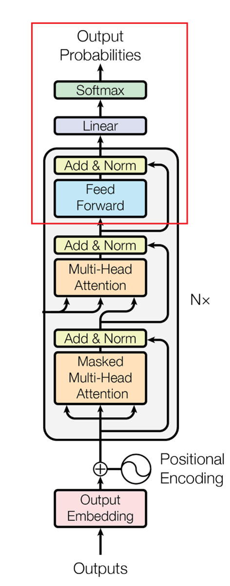
Image Source: Vaswani, A., et al. "Attention is all you need." Advances in neural information processing systems 30 (2017).
Upon receiving the concatenated output vectors from the previous stage of the Transformer model, these vectors are processed through a standard Feed-Forward Network, much like how vectors were handled in the Encoder block. The Feed-Forward Network typically includes two dense layers with an activation function applied between them. The objective of the Feed-Forward Network is to learn a non-linear mapping from input to output, transforming the vectors and altering their representations. The specific transformation of the vectors depends on the Feed-Forward Network's architecture and parameters. The next step involves feeding the transformed vectors into a crucial final linear layer.
After passing the initial vectors through the Feed-Forward Network you obtain modified versions of them, which are fed into a unique Final Linear layer. Following the Feed-Forward Network in a Transformer model, this linear layer generally has many neurons equivalent to the target language’s vocabulary size. In this English-French language example case, it will have as many neurons as there are unique words in the French vocabulary. This Final Linear layer aims to generate a probability distribution over the target vocabulary, representing the model's prediction for the next word in the sequence. This is achieved by computing a dot product between the Feed-Forward Network's output and a weight matrix, followed by a bias addition and a Softmax activation function. The resulting probability vector is used to sample the next word in the sequence during training or to select the most probable word during inference.
How Does the Transformer Model Perform Translation
Language translation for Machine Learning models involves predicting the next word in a sequence using two information sources: the original sentence and previously translated words. To translate, the model predicts the first word based on the original sentence and then predicts subsequent words using both the original sentence and previously predicted words. Masked Attention in the Decoder block is crucial to prevent the model from accessing information about future words, ensuring it learns effectively.
This process uses special tokens called the Start-Of-Sequence (SOS) and End-Of-Sequence (EOS) tokens. The SOS token marks the beginning of a sentence and serves as the first input to the Decoder in Transformer models. The EOS token, on the other hand, signifies the end of the translated sequence, indicating the model should stop generating words.
Both the SOS and EOS token vector values depend on the specific implementation. The original Transformer model represents these tokens as learned embedding vectors with the same dimensionality as the input sequence word embeddings. The embedding vectors for SOS and EOS tokens are initialized randomly and learned during model training along with other model parameters. By incorporating SOS and EOS tokens, the model can effectively generate cohesive and complete translations.
Consider my example English sentence, "The dog barked at the cat," and its French translation, "Le chien a aboyé au chat." In the French language translation, the model predicts the next word in the sequence using two information sources: the original sentence (English) and the translated words so far (French).
First, the model receives the SOS token, which indicates the start of the translation. Based on the original sentence and the SOS token, the model predicts the first French word, "Le." Next, it uses the original English sentence and the predicted word "Le" to predict the second French word, "chien." This process continues to use both the original sentence and previously predicted French words to generate the subsequent words: "a," "aboyé," "au," and "chat." The EOS token signifies the end of the translated sequence, indicating the model should stop generating words. Once the model predicts the EOS token, the translation is complete.
What Are the Differences Between the Original Transformer Model and GPT?
The original Transformer architecture spawned two very popular variants of it: the Generative Pre-trained Transformer (GPT) model and the BERT model. GPT, developed by OpenAI, generates human-like text using a pre-trained language model that excels in long text sequences while maintaining accuracy and coherence. GPT can perform various tasks such as translation and summarization. BERT, created by Google’s AI Language team, processes text bi-directionally, improving context understanding and outperforming traditional Natural Language Processing (NLP) models.
In terms of architecture, BERT is a model you create by stacking the Encoder parts of the Transformer architecture, while GPT is what you get when you stack the Decoder parts of the Transformer architecture. ChatGPT is part of the GPT family, but it is not the first model in that family, nor is it an exact copy of the Decoder block used in the original Transformer architecture.
The architecture of the original GPT model consists of a stack of Transformer Decoder blocks. Basically, it is the result of putting multiple Decoder blocks one after the other. Compared to GPT-2 (Generative Pre-trained Transformer 2) and GPT-3 (Generative Pre-trained Transformer 3), the original GPT model has fewer parameters and is less complex. However, it still produces high-quality text and has been used in various NLP applications.
The architecture of GPT-2 is similar to the original GPT, but it is much larger and more complex. Like the original GPT, GPT-2 is based on a stack of Transformer Decoder blocks. However, GPT-2 has more layers and attention heads in each block, allowing it to better capture complex dependencies between words and generate more coherent and fluent text. In addition to the Transformer Decoder blocks, GPT-2 also includes several other features, such as layer normalization and residual connections, which help improve the model's performance.
GPT-3 is one of the largest language models ever created, with up to 175 billion parameters. The architecture of GPT-3 is like GPT-2 but with several enhancements and improvements. Including a more diverse set of pre-training tasks, GPT-3 can perform few-shot and zero-shot learning, and use a technique called "prompt engineering.” These improvements allow GPT-3 to generate more fluent and coherent text, and makes it one of the most advanced language models available today.
ChatGPT comes in between GPT-3 and the latest model released in the GPT family, the GPT-4 (Generative Pre-trained Transformer 4) model. You can consider it somewhat of a GPT 3.5 model. The main difference between ChatGPT and GPT-3 is not in their architecture but in how the two models were trained. ChatGPT was trained on a dataset of conversational data, which includes dialogue and chat logs, while GPT-3 was trained on a much larger and more diverse dataset of web pages, books, and articles. As a result, ChatGPT is better suited for generating natural and contextually relevant responses in a conversational setting, while GPT-3 is better suited for generating high-quality text in general.
GPT-4 is the newest model in the series, released on March 14, 2023. It is very different from the other models because it is a multimodal model, which means it can take in both images and text inputs even though it can only generate text outputs. Because of how new it is, there is still not enough information on GPT-4 to go further in-depth.
- Intro to Image Augmentation: What Are Pixel-Based Transformations?
- Intro to Image Augmentation: How to Use Spatial-Level Image Transformations
The Decoder block plays a pivotal role in the Transformer architecture, which is widely regarded as a game-changing development in NLP. The Decoder is responsible for generating the output sequence, which is crucial in machine translation and text generation tasks. The Transformer architecture has evolved over time and one of its most popular variants is GPT, which has revolutionized language modeling. In this article, I explained the Decoder block of the Transformer model, building on the explanation in the previous article that focused specifically on the Encoder block. I also explained how the Transformer model performs language translation, and the difference between a standard Transformer model and a GPT model.

![[Future of Work Ep.5] The Future of Marketing with Zach Braiker: Personalize, Personalize, Personalize](https://res.cloudinary.com/edlitera/image/upload/ar_16:9,c_fill,f_auto,q_auto,w_100/dvaqyx9hepk27o8ya1hizvttxvww?_a=BACJ3SGT)