The precursors to modern diffusion models are worth mentioning and explaining, before diving deep into what is diffusion and how modern diffusion models work. These precursors are Variational Autoencoders (VAEs) and Generative Adversarial Networks (GANs). Both VAE and GAN models belong in the category of generative models, despite their evident architectural differences. Let us explain how each of these two models works individually to gain a deeper understanding of them. Afterward, we can jump directly into diffusion in the following article of this series.

What Are Variational Autoencoders

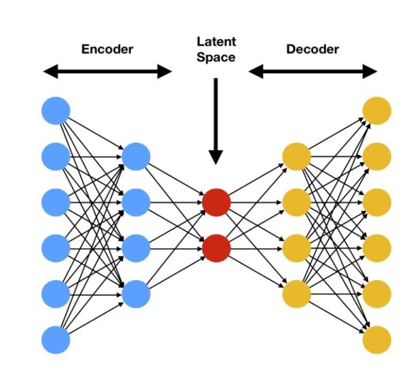
The architecture of a VAE model is, at least upon first impression, similar to the architecture of standard Autoencoders. After all, they also consist of three main parts:

•  The encoder part 
•  The latent space
•  The decoder part

However, even though the general architecture is mostly the same, the way we process data is slightly different. 

The encoder in standard autoencoders encodes our input data. It takes the data (e.g. an image) and maps it to a lower-dimensional latent space representation. The latent space can be considered as a compressed form of our input data, effectively encompassing all of the important characteristics and patterns. This is true even in its compressed state. This compressed version of our data will then be used as input to the decoder. The decoder attempts to reconstruct the original image from it. The higher the quality of the image reconstruction by the model, the better the autoencoder performs. In general, we use the Mean Square Error (MSE) as our loss function. It allows us to measure how well the decoder can reconstruct the input. 

• Intro to Transformers: The Encoder Block
• Intro to Transformers: The Decoder Block

While VAE models generally employ the same architecture, they introduce a few changes. These changes enable them to function as full-fledged generative models. To be more precise, we define the latent space differently, as well as use a different loss function. Unlike the latent space used in standard autoencoders, the latent space in Variational Autoencoders is probabilistic, instead of deterministic. The meaning of this can easily be explained in a simple way, with no need for complex math. 

Imagine you have a black-and-white image of a smiling face. In a standard autoencoder, the model could learn a fixed set of numbers to represent this image in the latent space. Let us assume the model learns the numbers (0.3, 0.8, -1.2) to represent this smiling face. These numbers will remain the same every time you input the same smiling face.

Now, in a Variational Autoencoder, the model does not only learn a fixed set of numbers for the smiling face. Instead, it learns a probability distribution over the latent variables. Therefore, for the same smiling face, it can be learned that the latent space consists of a range of possibilities. In other words, for the same smiling face, we can get several different values like (0.1, 0.6, -0.9) or (0.3, 0.8, -1.1) on different runs or samples from the model.

• How to Detect Emotions in Images Using Python

The ability to map the same image to multiple different values from the same probability distribution is an important aspect of Variational Autoencoders. It allows the model to generate similar but not completely identical images of smiling faces. This is done by sampling different points within the probability distribution.

The other difference between standard autoencoders and VAEs lies in the loss function. The loss function in a VAE is composed not only of the reconstruction loss but also of the regularization term we add to it. The regularization term encourages the latent space to follow a specific probability distribution. Usually, this distribution is a Gaussian distribution with mean 0 and variance 1. 

As networks, VAEs are mainly used for synthetic data creation and data augmentation. However, they are also applied in various other domains such as image denoising and deconstruction, feature extraction, and dimensionality reduction.

What Are the Advantages of VAEs 

The main advantages are: 

• The ability to  produce highly diverse outputs
•  No need for a great amount of computational resources
•  Using them for more than just synthetic data creation thanks to their way of working 

 What Are the Disadvantages of VAEs 

The main disadvantages are:

• The low-fidelity outputs produced in comparison to other generative models
• Highly sensitive to even the slightest changes in hyperparameter values
• One potential issue arises when the generative model struggles to encompass the diversity of the input data distribution. Instead,  it repeatedly produces highly similar or identical outputs, for example  into mode collapse

From the aforementioned, the lower fidelity of the generated samples seems to be the most serious problem. This is because other models, such as GANs, also suffer from mode collapse from time to time.

What Are Generative Adversarial Networks

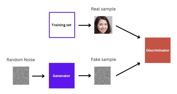
Generative Adversarial Networks, also known as GANs, were revolutionary at the time of their release. This is because they introduced a completely new approach to generating new data. A GAN consists of two neural networks:

•  Generator Network
•  Discriminator Network

These two networks are simultaneously trained in a zero-sum game. The Generator Network creates fake data, designed to mimic real data, and sends it to the Discriminator Network. The Discriminator Network receives this fake data, as well as several real data, and needs to distinguish between the two. Therefore, in essence, the Generator's objective is to produce data that is indistinguishable from real data. To put it simply, the aim is to trick the Discriminator. In contrast, the Discriminator learns to become more adept at distinguishing real data from fake data. This adversarial process continues until the Generator produces highly realistic data. In the realm of Computer Vision, this entails the generator's task of creating fake images. Conversely, the Discriminator's role is to distinguish between real images (from the training dataset) and fake images (produced by the Generator). 

Given the contradictory goals of the two networks involved, implementing GANs presents a challenge in devising an effective loss function. In the seminal paper introducing GANs, the Minimax Loss function was employed—a version modified for enhanced performance. This function operates under a straightforward concept. On the one hand, the Discriminator aims to maximize its accuracy in identifying real versus fake data. On the other hand, the Generator strives to minimize the Discriminator's success rate by improving the quality of its synthetic outputs. The modified version of this loss function introduced adjustments to the learning algorithm. This ensures that the networks continue to improve and avoid stagnation, a common issue with the original Minimax approach. 

In more recent developments, advanced loss functions have been introduced. An example of this is the Wasserstein loss. These modern adaptations are designed to refine further and optimize the training process of GAN architectures. This enables more sophisticated and efficient generation of synthetic data.

As networks, GANs are mainly used for synthetic data creation and data augmentation. However, they can find applications in many other areas, including art, fashion, design, etc. 

• Intro to Image Augmentation: What Are Pixel-Based Transformations?
• Intro to Image Augmentation: How to Use Spatial-Level Image Transformations

What Are the Advantages of GANs 

The main advantages are:

• GANs are capable of producing high-resolution, realistic images, surpassing many other generative models in quality.
• The wide range of applications, from art creation to synthetic data creation
• No need for labeled data
  
  

What Are the Disadvantages of GANs

The main disadvantages are:

• The training difficulty is because they require the training balance  of two neural networks
• The requirement of significant computational resources
• The results are not as varied as the ones produced by VAEs

Here is a simple example of how we train a GAN to create images of people's faces. 

Initially, the Generator will not know how to utilize the random noise provided as input and will more or less send something similar to the Discriminator. Therefore, the Discriminator can easily tell which image is real, and which is fake.

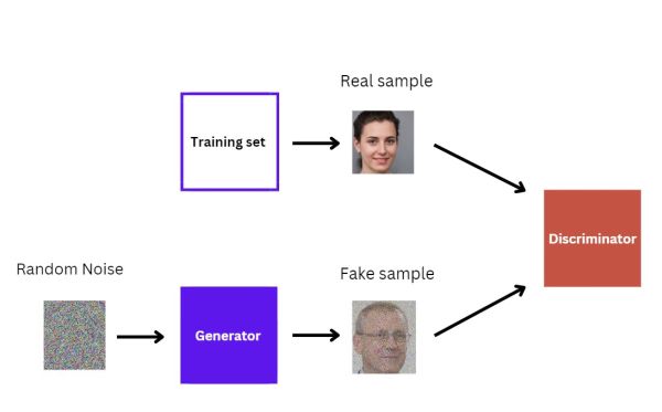
However, through multiple iterations, the Generator will improve at creating fake samples. At this point, the model still has not finished training because the Discriminator can still differentiate between real and fake samples.

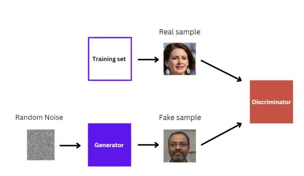
Finally, after experiencing many iterations, the Generator will start producing images of extremely high quality. As a result, the Discriminator will be unable to differentiate between the real and the fake.

At this point, our GAN has finished training because the Discriminator can no longer recognize which image is real, and which one is not.

• How to Evaluate Classification Models
• How to Evaluate Regression Models

Both VAEs and GANs were, when they first came out, considered to be the best generative models out there. However, nowadays they are no longer used as much as diffusion models because diffusion models outperform them in many aspects. Anyhow, their importance lies in being considered precursors to modern diffusion models. Now that we have covered the basics of these two types of networks, we can shift our focus to diffusion models in the following article of this series.