


Table of Contents
Despite the recent buzz, machine learning operations, or MLOps for short, is not really a new idea or a new field. The idea of focusing more on how to optimize machine learning in production was first introduced in a 2015 paper, Hidden Technical Debt in Machine Learning Systems. Even though this paper vividly described a number of challenges that need to be overcome when deploying machine learning models in production, newcomers to the field of machine learning rarely need to think about these barriers that advanced users of machine learning face.
First, be sure to check the Introduction to MLOps article to get a more detailed look into the field of MLOps. In this article, I will discuss why new data scientists rarely dive deep into this field.
Why You Should Learn MLOps
A lot of people who are interested in data science try to take the quick route. Becoming a data scientist is not easy, and even with proper guidance, it requires a lot of effort and a lot of knowledge in a number of different fields. This combination of high levels of interest in the field of machine learning along with newcomers who have little of the prerequisite knowledge needed to understand machine learning has become the main reason why most machine learning engineers never get to become MLOps specialists.
Starting from scratch means focusing time and effort learning the fundamentals, and then gaining as much experience as possible. This leaves little time to focus on the two other important parts of MLOps: DevOps and data engineering.
To facilitate MLOps as much as possible and simplify the problems getting into it, an abundance of different tools have become relatively easily accessible. Some of these tools are easier to use than others but offer little in terms of flexibility and adjustability. There are also tools that are very powerful, but are hard to use. MLflow hits the sweet spot somewhere in the middle of that spectrum.
As an open source platform, it is easy to come by and relatively easy to use while still being very powerful and flexible as an MLOps tool. Since it is not a completely new tool, most of the initial problems that come along with new tools have been fixed. This combination of reliability and ease of usage, along with the fact that it is also a powerful tool, means that MLflow is one of the top solutions for managing almost the whole lifecycle of a machine learning project. Let's dive deep into MLflow and explain why it is one of the most popular MLOps tools.
What is MLflow
MLflow is a tool for managing the lifecycle of machine learning models. It was created by a proven and accomplished team. Its creators are also behind both the popular cloud platform Databricks and the even more popular unified analytics engine Apache Spark. This should instill confidence into anyone looking to use MLflow for their MLOps needs. MLflow was first released with three main components, with a fourth being added relatively recently. Those four main components are:
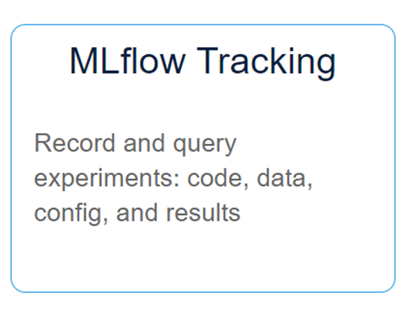
- MLflow Tracking
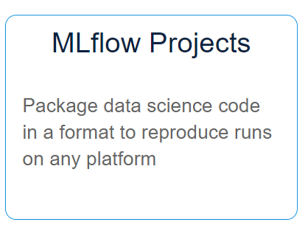
- MLflow Projects
- MLflow Models
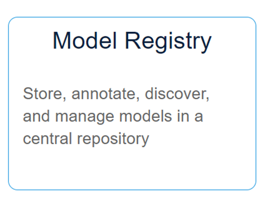
- Model Registry
Each of the components aims to cover an important aspect of machine learning development. A plethora of problems appear at each step, but they can generally be boiled down to:
- Number of tools needed to cover every aspect of the ML lifecycle
- Ease of integration
- Reproducibility
- Reliability
- Scalability
- Problems with governance
- Problems with team member cooperation
MLflow tries to solve all of these. Prizing itself on being both open source and open interface, MLflow indeed manages to deal with many (if not all) problems that present themselves during an ML model lifecycle. Even if a problem that it can't solve arises, a more specialized solution for that problem can be implemented because MLflow is so easy to integrate with a large number of different tools. Being able to solve most problems while also being easy to integrate with tools that can solve remaining problems seems to be a winning combination, and why MLflow is used by many MLOps teams.
Article continues below
Want to learn more? Check out some of our courses:
What Are the Components of MLflow?
Let's analyze and explain in detail the four main components of MLflow and how they are connected.
MLflow Tracking
MLflow Tracking simplifies the process of tracking. Aside from creating logs for code versions, parameters and metrics, it can also be used as a means of creating output files. It is characterized by how easy it is to use. Following the concept of so-called runs, the MLflow Tracking component can be called to log and query using REST or Python. It is especially practical for individuals who have experience creating machine learning models but don't have any experience properly managing them. The UI of MLflow Tracking is very straightforward. The inclusion of such a UI is actually the main driving force behind easily tracking a lot of different aspects connected to machine learning models. However, a good UI would mean nothing if the code for this component of MLflow was hard to implement.
Fortunately, adding MLflow Tracking to your existing code is very easy. A few lines of code allow you to build a whole tracking framework that will keep logs of everything that is important to you for managing machine learning models. To finish off, I must mention one additional thing: visualizations.
Visualizing metrics is achieved easily with the UI. That in turn allows you to compare different runs and choose the best one with relative ease. This component of MLflow offers great and flexible solutions for teams of all sizes. Even a single user can find many benefits to tracking machine learning models using this component. This scalability means that MLflow is very easy to use.
MLflow Projects
This component is based on the concept of projects. This is not something new. The idea of packaging code so that it can be used by others in a reproducible manner is something programmers have been using for a long time now. Similar to how packaging code usually works, MLflow Projects enables the creation of packages of reusable data science code. Those projects take the form of simple directories or even Git repositories.
Each project is defined by a YAML file. This file defines what is needed to run the code and how to run the code. Another thing that should be mentioned is that MLflow Projects allows you to create workflows by chaining together multiple projects. Combining the API for MLflow Projects with MLflow Tracking allows the user to create some form of a pipeline. Workflows are created by connecting separate projects together into one big multistep workflow.
Projects are very useful in terms of packaging code, but there are better solutions to building pipelines than chaining projects to each other. Usually, companies work with different technology stacks, so what you will choose depends on what stack you are using. For example, companies that use AWS will probably combine MLflow with SageMaker in their solutions.
If you are looking for the simplest solution, Databricks provides a version of MLflow that is fully managed and hosted. That is to be expected considering that Databricks created MLflow.
MLflow Models
Models in MLflow are packaged inside the MLflow Model format. The innovation that makes dealing with models easier is called flavors. These flavors remove the need for standard types of tool integration. Instead of integrating each tool with each library, flavors serve as conventions that allow deployment tools to understand how ML models work. These flavors cover both standard functionalities and custom ones.
For example, there is a Python function flavor that makes running a model as easy as running a simple Python function. On the other hand, there are also custom flavors connected with certain libraries, such as Scikit-learn, SageMaker. Every model is defined by an MLflow model YAML format file which holds all the necessary flavors that are needed for that specific model. However, this YAML file is not enough to describe the model properly. To describe the model in more detail, you should add additional metadata in the form of:
- Model Signature - stores a signature that describes a model's inputs and outputs in the JSON format
- Model Input Example - holds an example valid input
This component may be the most important part of MLflow. It allows you to package models in an easy way and makes using different deployment tools fast and simple because flavors remove the need for integrating each tool with each library.
Model Registry
This component is the newest addition to MLflow. Before it was released, MLflow was missing one crucial thing: a governance system. That problem was solved by releasing Model Registry. Although some improvements can still be made, it covers the essential parts that are needed, such as:
- Model Lineage
- Model Versioning
- Stage Transitions
- Annotations
By looking at what Model Registry covers, one can conclude that it basically serves as a centralized model store. As a component, it also includes a set of APIs and a UI. Those are the two ways one can interact with Model Registry.
With the addition of the Model Registry component, MLflow has become the closest thing to an open-source end-to-end solution for doing MLOps. Although there are some improvements that still need to be made, MLflow’s shortcomings can easily be dealt with by using a few complementary tools, most of which are already offered on the Databricks platform.
How to Use MLflow for MLOps: An Example
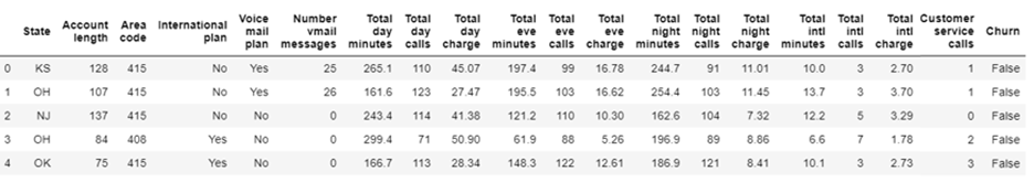
To learn how MLflow can be used for MLOps, next, you are going to work with the "Telecom Churn" dataset. This is a publicly available dataset that can be downloaded from Kaggle. You shouldn't focus too much on preparing the data since this dataset is relatively clean, but you will go through the process of initial analysis and cleaning before you will start using MLflow. The code will be written inside a Jupyter notebook to make this demonstration as easy as possible to follow.
How to Prepare the Data
After downloading this dataset, the first thing you need to do is make sure that you have all the necessary libraries that you are going to use for the purposes of this demonstration. You won’t use too many different libraries.
The ones you are going to use are:
- Pandas
- Scikit-learn
- XGBoost
- MLflow
All of these are easy to install using pip. After making sure the necessary libraries are available, you can start coding. To start off, you need to import all the libraries you are going to use in this notebook. You should always do this in the beginning to make sure your code stays as clean as possible.
1. # Import necessary libraries
2.
3. import pandas as pd
4.
5. from sklearn.model_selection import train_test_split
6. from sklearn.preprocessing import MinMaxScaler
7. from sklearn.metrics import roc_auc_score
8. from sklearn.metrics import roc_curve,auc
9. from sklearn.metrics import accuracy_score, classification_report
10. from sklearn.linear_model import LogisticRegression
11. import xgboost as xgb
12. from xgboost.sklearn import XGBClassifier
13.
14. import mlflow
15. from mlflow import pyfunc
16. import mflow.xgboost
Once you have imported everything you need, you can go ahead and:
- Load in your dataset using the pandas library
- Create a DataFrame
1. # Load in data
2.
3. churn_data = pd.read_csv("telecom_churn.csv")
As I mentioned earlier, before you implement MLflow, you need to do some initial data analysis and initial data cleaning.
First, you should take a look at a snapshot of the DataFrame using the head method from pandas:
1. # Display snapshot of the dataframe
2.
3. churn_data.head()
By running the code above, you will get:
Image Source: Edlitera
It seems like there is a mix of numerical and categorical data in this dataset. You need to take this into account going forward because you are going to use Scikit-learn models, which only take numerical values as inputs.
You can also see that the column names are problematic. You need to get rid of the white spaces between words and you need to make the column names lowercase.
Let's do that now:
1. # Remove white spaces and lowercase names
2.
3. churn_data.rename(columns=lambda x: x.replace(' ', '_').lower(), inplace=True)
Continuing with the initial analysis and cleaning, you should check whether there are duplicates present in your data.
Duplicates can be very problematic, so you need to deal with them as soon as possible:
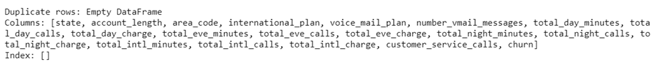
1. # Select duplicate rows
2.
3. duplicate_rows_data = churn_data[churn_data.duplicated()]
4. print(f"Duplicate rows: {duplicate_rows_data}")
The resulting output you should get from the code above is:
Image Source: Edlitera
There don't seem to be any duplicates inside this DataFrame. This assures you that the results you get using other pandas methods will be reliable.
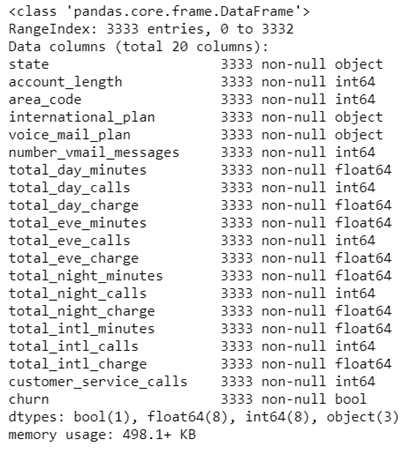
The next step will be to take a look at your dataset's basic information using the pandas info method. Looking at the info of a dataset is crucial for understanding how you will approach dealing with that dataset. Also, it dictates which preprocessing steps you need to do before you start building and training models.
1. # Get dataset information
2.
3. churn_data.info()
The information you get by using that method looks like this:
Image Source: Edlitera
Aside from giving you some insight into the different data types you need to work with, this method will also tell you if you are missing some data.
At first glance, it seems like there are no missing values in any of your columns, but to make sure, let's create a function that will check for missing values and then print out a DataFrame that represents the number of missing values and the percentage of missing values for each column in your dataset:
1. # Define a function that will check for missing data
2.
3. def analyze_missing_data(data):
4.     total_missing = data.isnull().sum().sort_values(ascending=False)
5.     percent_missing = data.isnull().sum() / data.isnull().count() * 100
6.     percent_missing.sort_values(ascending=False, inplace=True)
7.     missing_data_analysis = pd.concat(
8.         [total_missing, percent_missing],
9.         axis=1,
10.         keys=['Total', 'Percentage']
11.     )
12.
13.     return missing_data_analysis
14.
15. # And let's use that function to analyze missing data in our dataframe
16.
17. analyze_missing_data(churn_data)
The DataFrame created using the analyze_missing_data function should look like this:
This reaffirms the results of the info method. You could continue with analyzing the plausibility of your data and performing some EDA, but since that is not the focus of this article, I am going to skip that.
Next, you will need to create a function that will do the necessary preprocessing. I am going to incorporate some dataset preparation and data scaling into this function. This is something you would want to avoid doing manually. It is very impractical to clean and scale your data each time you want to use a new batch of data to train your models.
Let’s follow these steps:
- Create two lists: one of the numerical columns, the other of the categorical ones.
- Define the scaler you are going to use.
- Shuffle your data and then separate the dependent variable from the independent ones.
- Encode your dependent variable and transform it into a binary one instead of a boolean.
- Create datasets.
The code for the first step is:
1. # Create lists of numeric and categorical columns
2.
3. churn_numeric_columns = list(churn_data.select_dtypes(exclude=["bool_",
4. "object_"]))
5. churn_categorical_columns = list(churn_data.select_dtypes(exclude=["bool_",
6. "number"])
This will create the two lists that you are going to need later when you create your preprocessing function. You can go ahead and define the scaler you are going to use:
1. # Define scaler
2.
3. scaler = MinMaxScaler()
The MinMax scaler is an excellent choice to scale data. You want to make sure that the variables with bigger values don't snuff out the importance of the variables that have smaller values.
The code for your third preliminary step is:
1. # Shuffle data
2.
3. churn_data = churn_data.sample(frac=1).reset_index(drop=True)
4.
5. # Separate dependent varaible from independent varaibles
6.
7. X = churn_data.drop(columns=["churn"], axis=1)
8. y = churn_data["churn"]
Your dependent variable is now separate from your independent variables. However, you still need to deal with the fact that the data type of y is bool. The easiest way to deal with this is to just encode y as a binary variable. True will be equal to 1, and False will be equal to 0.
The code that changes the type of your dependent variable is:
1. # Convert boolean value into a binary one
2.
3. y = y.astype(int)
To finish off your preliminary tasks, you should use the train_test_split function from Scikit-learn to separate your data into training data and testing data:
1. # Create datasets
2.
3. X_train, X_test, y_train, y_test = train_test_split(X,
4.                                                     y,
5.                                                     train_size=0.8,
6.                                                     test_size=0.2,
7.                                                     random_state=1)
The prerequisites for creating your preprocessing function have been met. Let's create two versions of your preprocessing function. They are mostly the same. The only difference lies in how the data is scaled.
First, you will create the function that preprocesses your training data:
1. # Training data preprocessing function
2.
3. def train_preprocessing(df,
4.                 numeric_columns,
5.                 categorical_columns,
6.                 scaler):
7.
8.     new_churn = df[set(numeric_columns + categorical_columns)].copy()
9.     new_churn[numeric_columns] = scaler.fit_transform(new_churn[numeric_columns])
10.     churn_dummies = pd.get_dummies(new_churn[categorical_columns], drop_first=True)
11.     new_churn = pd.concat([new_churn, churn_dummies], axis=1)
12.     new_churn.drop(categorical_columns, axis=1, inplace = True)
13.
14.     return new_churn
Now you can create the function that preprocesses the data you will use for testing your models:
1. # Testing data prepreocessing function
2.
3. def test_preprocessing(df,
4.                 numeric_columns,
5.                 categorical_columns,
6.                 scaler):
7.
8.     new_churn = df[set(numeric_columns + categorical_columns)].copy()
9.     new_churn[numeric_columns] = scaler.transform(new_churn[numeric_columns])
10.     churn_dummies = pd.get_dummies(new_churn[categorical_columns], drop_first=True)
11.     new_churn = pd.concat([new_churn, churn_dummies], axis=1)
12.     new_churn.drop(categorical_columns, axis=1, inplace = True)
13.
14.     return new_churn
Now that you have prepared the two functions, let's preprocess the data:
1. # Preprocess training data
2.
3. X_train = train_preprocessing(X_train,
4.                               churn_numeric_columns,
5.                               churn_categorical_columns,
6.                               scaler)
7.
8. # Preprocess testing data
9.
10. X_test = test_preprocessing(X_test,
11.                             churn_numeric_columns,
12.                             churn_categorical_columns,
13.                             scaler)
With this, you have prepared everything you need to go through the four-part process of MLflow explained earlier in this article.
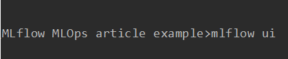
How to Set up and Use MLflow
After preparing everything you need for preprocessing your data, you can experience how MLflow Tracking works. To do that, you first need to run mlflow ui in your terminal.
As I mentioned earlier when I explained MLflow, you need to set up an experiment. To do that, you need to tell Python where to look, and define the experiment itself:
1. # Connect to MLflow
2.
3. mlflow.set_tracking_uri("http://localhost:5000")
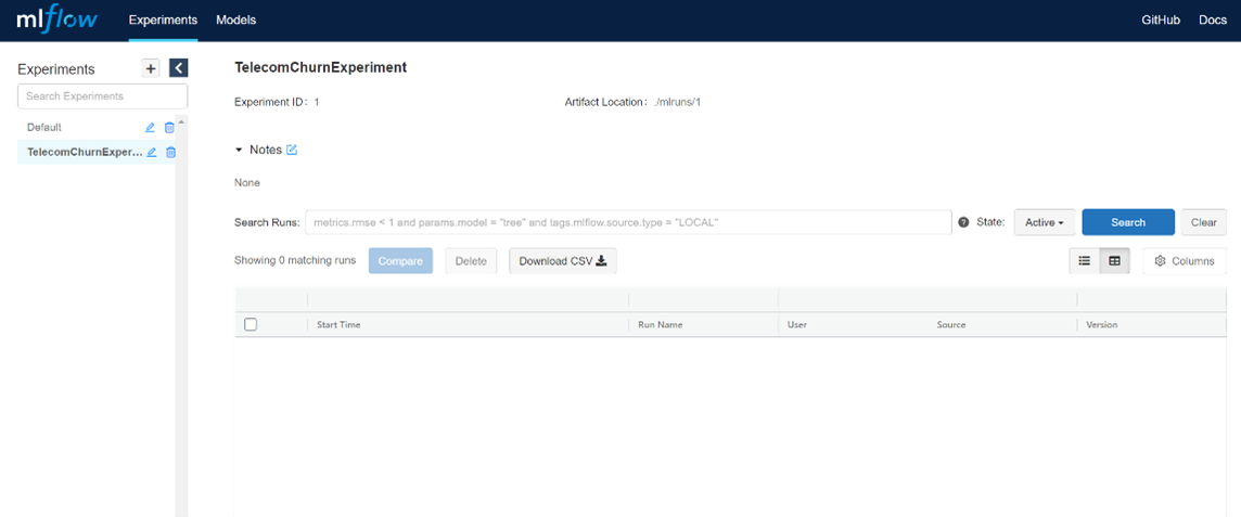
4. mlflow.set_experiment("TelecomChurnExperiment") Since only the default experiment exists for now, the result from running this code will be:

Following the link given in the tracking, if you open the UI it will look something like this:
Image Source: Edlitera
As you can see above, there are two experiments in the UI currently. One is the default experiment, and the other is the new experiment you just created. For now, both are empty since you haven't actually created a run.
To create a run, you are going to create a model using the default model interface for Python models: the python_function flavor. This is a good demonstration of MLflow Models, since it shows you can use flavors to create models. This format will allow you to easily package models. It is self-contained and holds everything needed to load and use a model. It also allows you to easily integrate any model from any tool. For the purposes of this demonstration, you are going to use two models: the Logistic Regression model and the XGBoost model. This way you will have two models to compare in your UI. Let's create the Logistic Regression model first.
To start off, you need to create a class that will define how your model looks. This will allow you to call on it later when you start creating runs. For the purposes of this example, you are going to create a very simple class. You just need to be able to track the results of your models. The code for creating such a class looks like this:
1. # Define model
2.
3. class Churn_Model(mlflow.pyfunc.PythonModel):
4.
5.     def __init__(self, model):
6.         self.model = model
7.
8.     def predict(self, context, model_input):
9.         return self.model.predict(model_input)
You can use this class for both the Logistic Regression model and the XGBoost model. You could define the environment so that you can later deploy the model on whichever platform you want.
Before going ahead with your first run, let's create a simple YAML file that defines the environment:
1. # define specific python and package versions for environment
2. mlflow_env = {
3.  'name': 'mlflow-env',
4.  'channels': ['defaults'],
5.  'dependencies': ['python=3.6.2', {'pip': ['mlflow==1.6.0','scikit-learn']}]
6. }
Getting back on track, let's create your first run, which will use a Logistic Regression model. The code above specifies the run with the Logistic Regression model. When coding, you first need to specify the parameters you want to use and the model you want to use.
Afterwards, since you want to check accuracy and the AUC score, you need to define how you calculate them. You can then define what you want to track and log. Then, you should save the run ID and experiment ID so you would have everything you need later on if you choose to deploy your model:
1. # Define and do run
2.
3. with mlflow.start_run(run_name="Churn Prediction model run 1") as run:
4.
5. # Define model parameters
6.
7. penalty = "l2"
8.
9. # Define model
10.
11. log_reg_model = LogisticRegression(solver='lbfgs', penalty=penalty)
12. log_reg_model.fit(X_train, y_train)
13.
14. y_pred_model = log_reg_model.predict(X_test)
15. predictions_test= log_reg_model.predict_proba(X_test)[:,1]
16.
17. accuracy = accuracy_score(y_pred_model, y_test)
18. auc_score = roc_auc_score(y_test, predictions_test)
19.
20. # Log parameters
21.
22. mlflow.log_param("penalty", penalty)
23.
24. # Log metrics
25.
26. mlflow.log_metric("accuracy", accuracy)
27. mlflow.log_metric("auc_score", auc_score)
28.
29.
30. # log model with all objects referenced
31.
32. pyfunc.log_model(
33. artifact_path = "churn_pyfunc",
34. python_model = Churn_Model(model=log_reg_model),
35. conda_env = mlflow_env)
36.
37. # Save run_id and experiment_id
38.
39. run_id = run.info.run_uuid
40. experiment_id = run.info.experiment_id
41.
42. # End run
43.
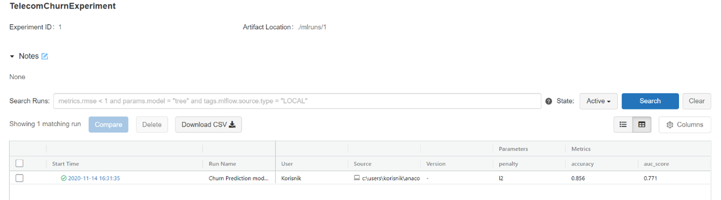
44. mlflow.end_run() After running the code, you can see your run by refreshing the page of the MLflow UI. You should switch the view mode to the compact one because you will have just two models in this demonstration:
Image Source: Edlitera
The results are relatively good.
Let's create the XGBoost run to demonstrate how you can compare them:
1. # Define and do run
2.
3. with mlflow.start_run(run_name="Churn Prediction model run 2") as run:
4.
5.     #Define model parameters
6.
7.     n_estimators = 1500
8.     learning_rate = 0.1
9.     max_depth = 4
10.
11.     # Define model
12.
13.     xgb_model = XGBClassifier(learning_rate=learning_rate,
14.                               n_estimators=n_estimators,
15.                               max_depth=max_depth)
16.
17.     xgb_model.fit(X_train, y_train)
18.
19.     y_pred_model = xgb_model.predict(X_test)
20.     predictions_test= xgb_model.predict_proba(X_test)[:,1]
21.
22.     accuracy = accuracy_score(y_pred_model, y_test)
23.     auc_score = roc_auc_score(y_test, predictions_test)
24.
25.     # Log parameters
26.
27.     mlflow.log_param("n_estimators", n_estimators)
28.     mlflow.log_param("learning_rate", learning_rate)
29.     mlflow.log_param("max_depth", max_depth)
30.
31.     # Log metrics
32.
33.     mlflow.log_metric("accuracy", accuracy)
34.     mlflow.log_metric("auc_score", auc_score)
35.
36.     # log model with all objects referenced
37.
38.     pyfunc.log_model(
39.         artifact_path = "churn_pyfunc",
40.         python_model = Churn_Model(model=xgb_model),
41.         conda_env = mlflow_env)
42.
43.     # Save run_id and experiment_id
44.
45.     run_id = run.info.run_uuid
46.     experiment_id = run.info.experiment_id
47.
48.     # End run
49.
50.     mlflow.end_run()
Let's take a look at the UI now:
Image Source: Edlitera
Notice that the XGBoost model performs much better.
The UI can also compare runs:
Image Source: Edlitera
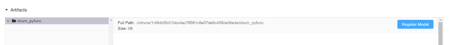
This option to compare runs is more useful when you have multiple runs with the same model but different hyperparameters. A potentially more useful option is looking at the details of the run with the XGBoost model. You can already see most of these details since any of the special tags and similar things were used, but you can also see the artifacts of that particular run.
Image Source: Edlitera
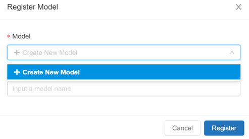
Here, you can easily see your model in the ML model format. You can also see the conda environment as a YAML file. When you have a run you are satisfied with, you can transition that run into a model in the MLflow Model Registry. You can do this by clicking on the upper right box in the artifacts section:
Image Source: Edlitera
It will then ask you if you want to create a new model.
Since you don't have a model, you will need to create a new one.
There is one potential problem that can arise. The models can't be saved anywhere you want. Basically, if you try to just save a run to the folder with your Jupyter notebooks, this error pops up:

Image Source: Edlitera
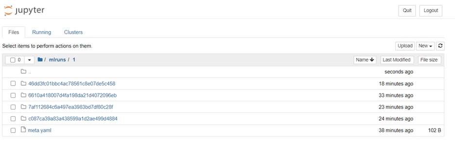
This means that you need to have a valid scheme to use the MLflow Model Registry. The reason for that is very simple, and can be seen in the image below:
Image Source: Edlitera
This is what a Jupyter notebook folder looks like after only 4 runs. Even if you tagged models perfectly and made sure that the names say the reason for a particular run, your folder would quickly become unusable. Because of that, some type of database system is necessary to house all of your runs.
This wraps up this demonstration of MLflow. The only aspect I didn't touch on is deployment. However, I will demonstrate that in the next article in this series, which explains the way you leverage AWS for MLOps, including model deployment via AWS. This is also the optimal way to deploy MLflow models.
In this article, I explained the four integral modules of MLflow. Using them, you can create, for the most part, a full machine learning workflow. Perhaps the best thing about MLflow is that it integrates so easily with other tools that it can cover its deficiencies very easily, which makes MLflow one of the most reliable tools for MLOps. Aside from its flexibility, it is relatively easy to use. Although it is not perfect, and needs some complementary tools (such as tools that will facilitate deployment), MLflow stands as one of the most complete options to choose from when deciding which platform to use for MLOps. Therefore, I recommend MLflow to every team that looks forward to creating their own MLOps workflow.
![[Future of Work Ep. 4]: The Future of Sales with Santosh Sharan: Is AI Coming for Sales Jobs?](https://res.cloudinary.com/edlitera/image/upload/ar_16:9,c_fill,f_auto,q_auto,w_100/6jyid1xo71je4h0n8xmoyllf2zjv?_a=BACJ3SGT)
