


Table of Contents
Understanding ensembles is essential to truly grasp the landscape of machine learning: they’re like the stepping stones that bridge basic models (like support vector machines, linear regression, and logistic regression) to more advanced territory. Diving straight into advanced techniques, like boosting algorithms and deep learning, without understanding ensembles will leave you with gaps in your foundational knowledge. To make sure your foundation is solid, in this article, I'll demystify ensembles and demonstrate how you can create them by merging multiple machine learning models. After reading this article, you'll know how to upgrade your models from single models to ensembles and achieve better results.
- What Are the Most Popular Machine Learning Service Tools in 2023?
- What Questions Can Machine Learning Help You Answer?
What Are Ensembles?
The idea behind ensemble learning is quite simple: instead of training a single model and relying on its prediction, you train multiple models and combine their predictions. This, in theory, gives you better overall accuracy.
Ensemble learning is useful because most models you create will be weak learners. Weak learners are models that do not outperform random guessing by a large margin, meaning they are not that useful on their own. Ensemble learning allows you to leverage the power of multiple weak learners by merging them into one larger model — you're essentially combining multiple weak learners to create a strong learner, a model that significantly outperforms random guessing.
Combining multiple weak learners yields a strong learner because each weak learner interprets data in a unique way, excelling in certain areas while faltering in others. Simply put, different models make different mistakes. In an ensemble setup, one model's strengths can compensate for another's weaknesses, ensuring the ensemble will produce an accurate prediction even if one of the models doesn’t produce an accurate prediction by itself. This is analogous to consulting a single expert versus consulting a panel of experts — advice from one expert can be helpful, but pooling advice from several experts produces more well-rounded insights.
Let’s look at ensemble learning from the perspective of machine learning. Imagine having a document that must be sorted into either class A or class B. You could train a single model and rely on its predictions, but in most cases, using multiple models is a much better idea. For instance, instead of training a single model, you can train five models and base your final prediction on the predictions of those five models. If a clear majority of them, say four models, suggest the document belongs to class A, the logical choice is to place the document in class A.
What I just described is one of the key aspects of ensemble learning: the voting ensemble method. Aside from voting ensembles, we can also create so-called bagging ensembles. Let’s look at these two types of ensembles in more detail.
Article continues below
Want to learn more? Check out some of our courses:
What Is the Voting Ensemble Method?
Voting is a popular ensemble learning method typically used in the context of classification. There are two types of voting:
- Hard voting
- Soft voting
What Is Hard Voting?
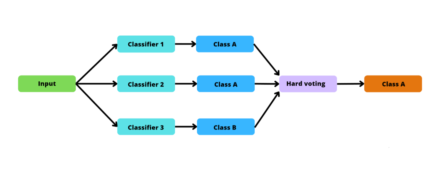
In hard voting, each model in the ensemble votes for one class, and the class that gets the majority of the votes is predicted as the output. For example, look at the following image. There are three classifiers: two classifiers voting for class A and one classifier voting for class B. Because we have two votes for class A and just one vote for class B, using hard voting, the ensemble will predict that the correct output should be class A.
A flowchart depicting the hard voting method.
Image source: Edlitera
What Is Soft Voting?
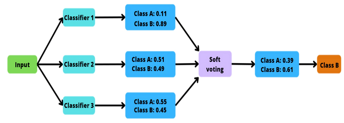
In soft voting, on the other hand, every classifier provides you with a probability value for each class and the class assigned with the highest average probability value is the predicted output. For example, look at the following image.
A flowchart depicting the soft voting method.
Image source: Edlitera
There are three classifiers that will give you a probability value for each class. Because there are only two classes, you’ll get a probability value for class A and a probability value for class B. To calculate the final probability value, you sum up the individual probability values and divide them by the number of classifiers.
In the example above, summing the probability values for class A for all three classifiers gives a value of 1.17. To get the final probability value for class A, you divide it by the number of classifiers, which is three, and end up with a value of 0.39. You can follow the same principle to get the final probability for class B.
After you have the final probability values, you just compare them and choose the best one. In this case, because the final probability for class B is bigger than the final probability for class A, we will predict class B. This, in a nutshell, is soft voting.
What Is the Bagging Ensemble Method?
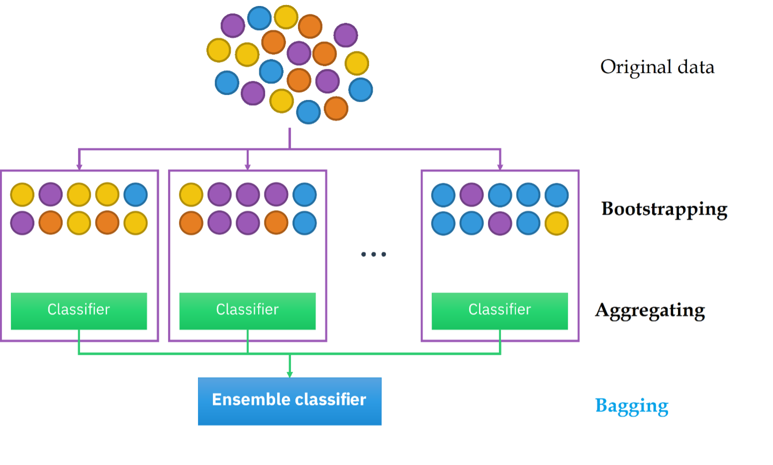
Bagging is a type of ensemble learning where you take several copies of the same model and train those copies on different samples of the original data. To get random samples, you perform random sampling with replacement, a.k.a., bootstrapping.
Bootstrapping creates multiple smaller training datasets from one bigger training dataset. By using bootstrapping, you make sure that every item has an equal chance of being chosen because you pick items from a group one at a time and place that item back in the group before picking from the group again. However, this also means you can end up with duplicates in your sample.
After creating these training datasets, you can train multiple models on them: the first model on the first dataset, the second model on the second one, and so on. In the end, you aggregate the predictions of your models to arrive at the ensemble's final prediction.
The bagging method.
Image source: Edlitera
A classic example of such a model is the random forest model. In the random forest model, you take the original data, perform bagging to generate multiple datasets for training, and then train a decision tree model on each sample dataset. In the end, you consolidate the predictions of the decision tree models to obtain the ultimate prediction of our random forest model.
How to Create an Ensemble in Python
Let’s demonstrate how to create ensembles by creating a voting ensemble. I won’t explain here how to make bagging ensembles, or a random forest model, because those merit an article of their own.
The first thing I am going to do is import everything I plan on using in this example:
# Import what we need
import pandas as pd
from sklearn.model_selection import train_test_split
from sklearn.preprocessing import StandardScaler
from sklearn.ensemble import VotingClassifier
from sklearn.linear_model import LogisticRegression
from sklearn.tree import DecisionTreeClassifier
from sklearn.svm import SVC
from sklearn.metrics import classification_report
After importing everything, I’ll load my data into a DataFrame. To do so, I will use the read_csv() function from Pandas, which allows me to load my data directly from an S3 bucket. After that, I can use the head() method to display the first five rows.
- Intro to Pandas: What Is a Pandas DataFrame and How to Create One
- Intro to Pandas: How to Analyze Pandas DataFrames
# Load the data into a DataFrame
data = pd.read_csv("https://edlitera-datasets.s3.amazonaws.com/iris.csv")

# Display the first five rows of our DataFrame
data.head()
The result I get by running the code above is:
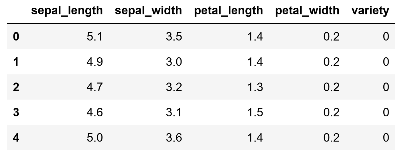
Image source: Edlitera
In this example, I am using the Iris dataset, which is a very famous dataset typically used to test out machine learning models. It’s a dataset consisting of five columns containing information about different species of iris flowers. The sepal_length, sepal_width, petal_length, and petal_width columns are independent features, while the variety column is the label. I’m going to train a model that will predict the variety of an iris flower based on its characteristics.
But first, I need to prepare the data for training the model. First, I will separate the independent features from the label. After that, I will use the train_test_split() function from Scikit Learn to separate the data into training and test data. I will use 20 % of the total data for testing and define a random state value to ensure that the results I get using this function are reproducible.
# Separate the independent features from the dependent feature
X = data.drop(columns=["variety"])
y = data["variety"]

# Split the dataset into a training set and a test set
X_train, X_test, y_train, y_test = train_test_split(X, y, test_size=0.2, random_state=1)
After I split the dataset into a training and test dataset, the data is almost ready — there is just one thing I need to do before feeding it into my model: scaling. This will ensure that all the features will be treated as equally important, and the differences in magnitude between their values won't bias the model. To scale the data, I will use the StandardScaler() from Scikit Learn. This scaler standardizes the features by removing the mean and scaling them to unit variance.
# Define the scaler
scaler = StandardScaler()

# Scale the features
X_train = scaler.fit_transform(X_train)
X_test = scaler.transform(X_test)
Remember, when scaling data, you always fit the scaler only on the training data, never on the test data. This way, you avoid data leakage, which is when information from the test set inadvertently influences the model during training. When preprocessing tools (e.g., scalers) are fit using the test set, they capture and expose statistical properties of the test data to the model. This can lead to overly optimistic estimates of a model's performance because the model has already "seen" the test data.
Next, let's create an ensemble that will consist of three models:
- Logistic regression model
- Decision tree model
- Support vector machine model
I will use the three classes we imported from Scikit Learn to create these models.
# Define the three models
# we will use in our ensemble
first_classifier = LogisticRegression()
second_classifier = DecisionTreeClassifier()
third_classifier = SVC()
After creating the three models, I can combine them into a voting ensemble by creating an instance of the VotingClassifier() class from Scikit Learn. For this demonstration, the ensemble will use hard voting to aggregate the predictions of the three models into a final prediction.
# Define the ensemble model
ensemble = VotingClassifier(estimators=[
    ("logistic regression", first_classifier),
    ("decision tree", second_classifier),
    ("support vector machine", third_classifier)
], voting="hard")
Now it's time to train the model. I will train it on the training dataset that I created and scaled earlier using the fit() method.
# Train the ensemble
ensemble.fit(X_train, y_train)
After the model has finished training, it is time to evaluate it. To do so, I am going to make predictions using the trained model with the predict() method and will then compare my predictions to the actual target values by creating a classification report using the classification_report() function from Scikit Learn.
# Use the ensemble to make predictions
predictions = ensemble.predict(X_test)
# Generate the classification report
report = classification_report(y_test, predictions)
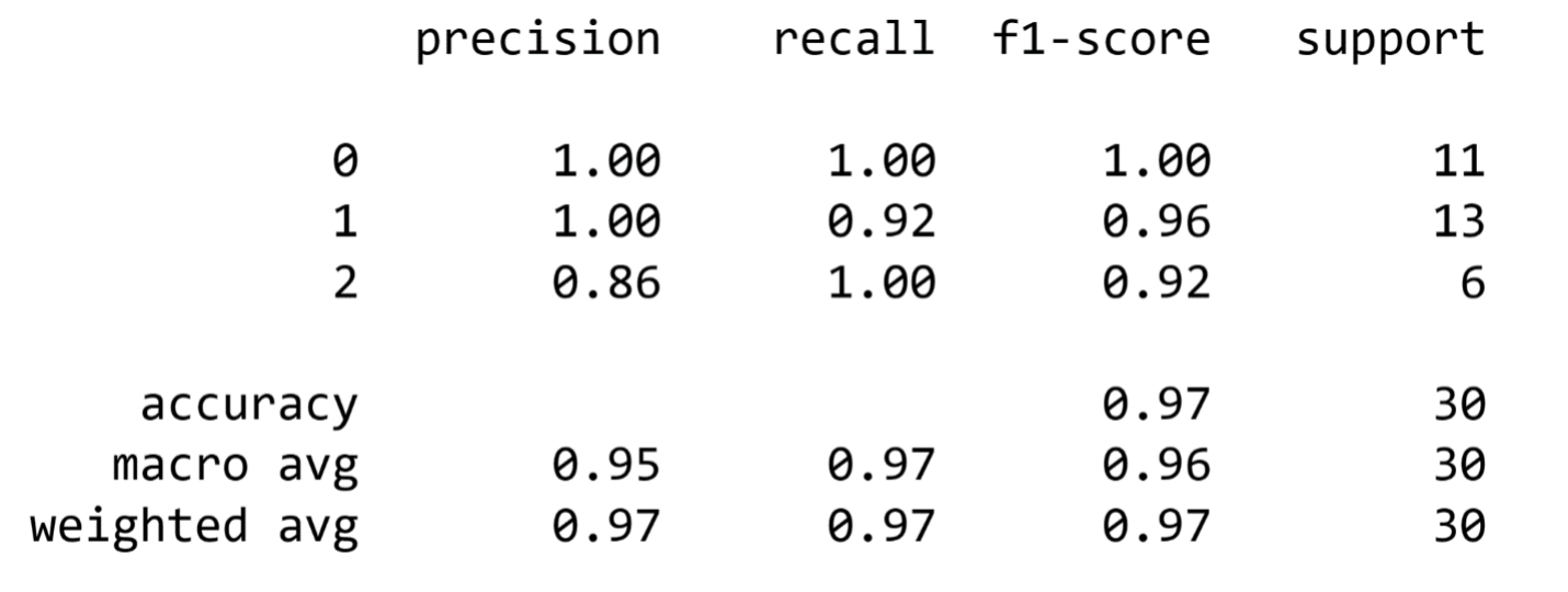
print(report)The result I get by running the code above is:
As you can see, the model is performing great — it achieves a weighted average F1 score of 0.97, which is excellent. If you wanted to further improve its performance, you could try and tune the individual models and deal with the obvious imbalance in the data, but that is outside the scope of this article.
Ensemble methods are pivotal techniques in the realm of machine learning. By harnessing the power of multiple models and intelligently aggregating their outputs, ensembles often outperform single models by a large margin, and they consistently deliver superior performance across a wide range of applications. In this article, I explained what ensembles are, why you should use ensembles, and how you can create an ensemble of machine learning models to solve a classification problem. Now you’re ready to start using ensembles in your projects.

