As one of the two most common tasks we typically solve with classic machine learning models, alongside regression, classification is a problem that a wide variety of algorithms can solve. While it is always best to try and solve a classification problem using simpler models such as logistic regression or support vector machines, in many cases, you need to use more complex models to solve problems. For example, Decision Tree algorithms can tackle both regression and classification tasks. In this article, I will explain their application in addressing classification problems.

 

• << Read previous article in the series: How to Evaluate Regression Models

 

Introduction to Decision Tree Classifiers

Decision Trees are very popular classic machine learning algorithms with a structure similar to flowcharts. They consist of three main elements:

 

• internal nodes
• branches
• leaf nodes

Decision Trees begin at the root node, where the data gets split based on specific rules and travels down branches to create more internal sub-nodes. This continues until you hit a leaf node, which shows the class or group the data belongs to. 

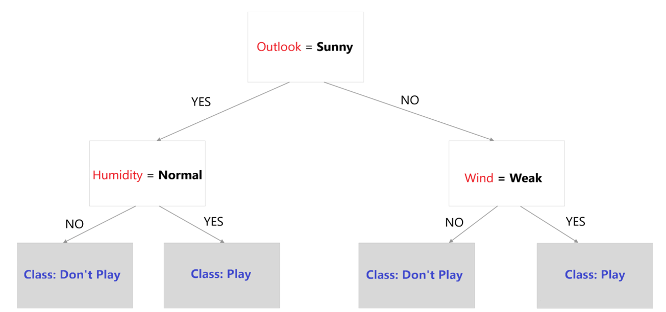
A decision tree.

Image source: Edlitera.

In the example above, the white rectangles represent the internal nodes, including the root node at the top and the sub-nodes on the lower levels, while the arrows represent branches. Additionally, each grey rectangle represents a leaf node. Using such a Decision Tree is very simple. 

Let's demonstrate how you can use a trained model to assign correct labels to data instances by using the following example data instance:  

Labelled data instances.

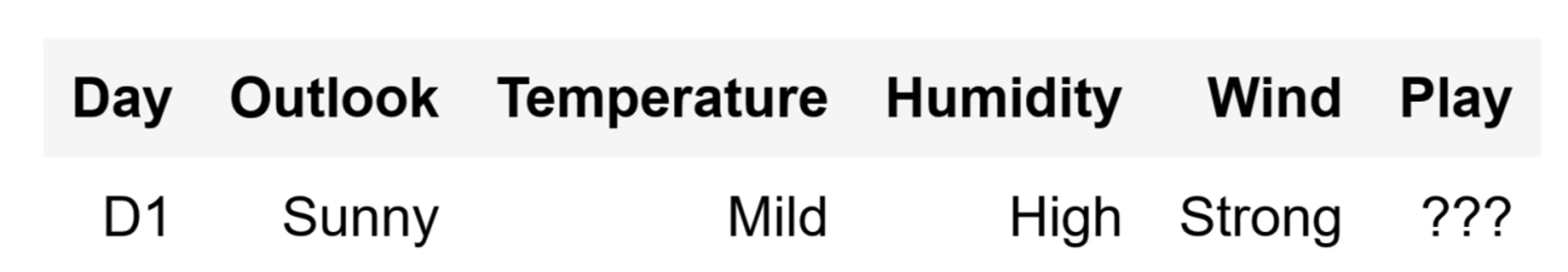
Image source: Edlitera.

The goal is to predict whether a child should play outside or not. Following the Decision Tree in the previous image, I can determine that the child should NOT play outside. How do I know this? Well, starting from the tree's root node, the split is on the Outlook feature, so I can check whether the outlook is sunny or not. Since it is sunny, I follow the YES branch to the next internal node on the left. Here, the data splits based on the Humidity feature. Because the humidity is high and not normal, I will follow the NO branch, which leads me to a leaf node that predicts that the child should NOT play outside.

As you can see, using a Decision Tree to make predictions is relatively easy. However, arriving at that Decision Tree is not. Training a Decision Tree model means trying out different combinations of these splits and tree structures until you find the one that best splits your data into the correct classes. At that point, if your model splits your training data with a high degree of accuracy, you can safely assume that when a new data point arrives, you can just push it through the tree flowchart, and it will arrive at the correct leaf node.

At this point, you might be wondering, "How do I know which potential split best splits my data?" After all, some internal nodes lead to other internal nodes and not to leaf nodes, which means that you can't determine the quality of the split by how many examples it correctly classified. Luckily, you can evaluate the quality of a split by calculating two metrics that tell you how well the particular "test" at an internal node splits data. These are:

 

• Gini Impurity
• Entropy

 

What Is Gini Impurity?

The Gini Impurity is a way to see how likely it is for a specific piece of data to be placed in the wrong group when picked out at random. To simplify, when you perform a split at an internal node, you want to make sure that all data points that follow a specific branch will be members of the same class because this, in turn, means that the data points following the other branch are also going to be members of the same class. Such a split would have a Gini Impurity of 0, so it would be completely “pure.” It would also mean that, at that point, your model is perfectly accurate because it splits data perfectly. In practice, the Gini Impurity is often higher than 0 but no higher than 1. A Gini Impurity of 1 denotes a completely "impure" split, meaning that the data points randomly follow the different branches, or in other words, our model guesses at random to which class a data point belongs. 

The equation to calculate the Gini Impurity is:

 

\( G=1-\displaystyle\sum_{i=1}^{n}(p_i )^2 \)

In the equation above,  p_i denotes the probability of an object being assigned to a particular class. When determining how good a split is, you have to calculate the value for each branch of the split and then weigh the impurity of each branch with how many elements that branch contains. A typical split might look like this:

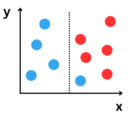
Data split on an internal node.

Image source: Edlitera.

Looking at the image above, the left branch has a value of zero because it only has blue samples.

\( G_{left}=1-((p_{blue})^2+(p_{red})^2 ) \)

\( G_{left}=1-((1)^2+(0)^2 )=0 \)

The right branch, on the other hand, doesn't have a value of zero because there is a mix of blue and red samples. Because the probability of drawing a blue sample from the right branch is 1/6, and the probability of drawing a red sample is 5/6, you can easily calculate the value as follows:

\( G_{right}=1-((p_{blue})^2+(p_{red} )^2 ) \)

\( G_{right}=1-((\frac{1}{6})^2+(\frac{5}{6})^2 )=0.2777777778 \)

Finally, to measure the Gini Impurity value of our split, you will weigh the calculated values. You need to do this because each branch likely has a different number of elements. You can calculate the weighted Gini Impurity values with the following equation:

\( G_{split}= G_{left}\times\frac{samples in the left branch}{total number of samples}+G_{right}\times\frac{samples in the left branch}{total number of samples} \)

In this case, when I plug in the numbers, the final result is:

\( G_{split}= 0\times(\frac{4}{10})+0.2777777778\times(\frac{6}{10})= 0.1666666667 \)

As you can see, the Gini Impurity of this split is very close to 0, which means that the split is excellent. Once you’ve calculated this value, you can compare it with the value achieved before this split to get the Gini Gain. The Gini Gain represents how much the impurity decreases when you use this split - the higher it is, the better. For example, let's say that the Gini Impurity achieved before the split was 0.5. Then you can calculate the Gini Gain as:

\( G_{gain}=0.5- 0.1666666667=0.3333333333 \)

By calculating the Gini gain value, you can easily determine whether your splits are improving or not. 

 

What Is Information Entropy?

Entropy measures how much "information" you get about a class using some feature. It is also often called Information Gain, but it is conceptually similar to Gini Gain. To get the Information Gain, you compare the Information Entropy before the split with the one after the split. To calculate the Information Entropy, you can use the following equation:

\( E=-\sum_{(i=1)}^np_i log_2 (p_i ) \)

Using the same example, the entropy of the left branch is going to be zero:

 

\( E_{left}=-1\times{log_2 (1)}=0 \)

On the other hand, the value for the right branch will once again be different from zero:

\( E_{right}= -(\frac{1}{6}  log_2(\frac{1}{6})+\frac{5}{6}  log_2(\frac{5}{6}) )=0.65002 \)

Again, you’ll need to weigh the values of each branch just as you did when calculating the Gini Impurity:

\( E_{split}= 0\times(\frac{4}{10})+0.65002\times(\frac{6}{10})= 0.390012 \)

That is the Information Entropy of the split. To get the Information Gain, you just determine how much entropy was removed by the split (the higher the number, the better). Once again, for demonstration, let's assume that the Information Entropy before the split was 0.5. The Information Gain would then be:

\( E_{gain}=0.5- 0.390012=0.109988 \)

 

When to Use Gini Impurity and When to Use Entropy

The choice between the two is mostly a matter of preference, but classic machine learning models use Gini Impurity by default for a simple reason: the results using both methods are nearly identical, but it is far less computationally expensive to calculate the Gini Impurity of a split than to calculate the Entropy of a split. Calculating the entropy requires the usage of logarithmic functions, which slows down the training of Decision Tree models without providing any benefits.

 

How to Use Classification Decision Trees in Python

By far the most popular classic machine learning learning library in Python is the Scikit Learn library. Fortunately, it also implements Decision Trees, both for classification and regression. Classification trees are non-parametric models and don't require much data preprocessing. However, because you’ll typically try out different models when trying to solve a problem, you will end up preprocessing the data before we feed it into a Decision Tree model.

 

• What Are the Most Common Types of Machine Learning Styles

Next, I’ll demonstrate how you can use the Decision Tree classifier from Scikit Learn to solve a classification problem. The dataset I will be using in this example is a modified version of a publicly available dataset that contains multiple features you can use to predict the likelihood of the progression from an initial incident indicating a potential occurrence of multiple sclerosis to a clinical diagnosis.

First, I need to import everything I will use in this example:

# Import what we need

import pandas as pd

from sklearn.tree import DecisionTreeClassifier

from sklearn.model_selection import train_test_split

from sklearn.metrics import classification_report

Then I need to load in my data and create a DataFrame using Pandas. I will use the read_csv() function from Pandas to load the CSV file that contains the data directly from where it is stored by referencing the link that leads to it. After I load the data and create a DataFrame, I will take a look at the first five rows using the head() method from Pandas.

 

• The Ultimate Python Pandas Cheat Sheet
• Intro to Pandas: What Is a Pandas DataFrame and How to Create One?
• Intro to Pandas: How to Analyze Pandas DataFrames

# Import the data and create a DataFrame

# Take a look at the first five rows

link = "https://edlitera-datasets.s3.amazonaws.com/multiple_sclerosis_prediction_dataset.csv"

df = pd.read_csv(link)

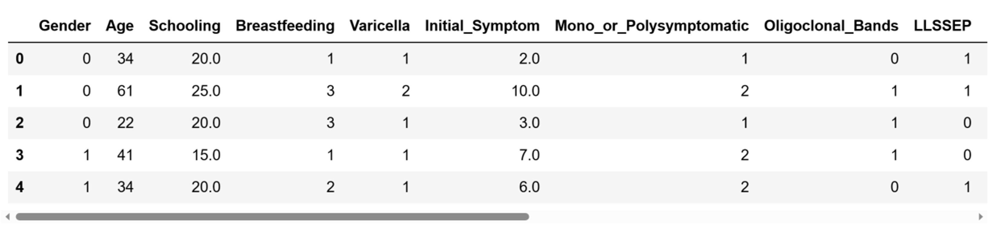
df.head()

The first five rows of the DataFrame I just created look like this:

Five first rows of the DataFrame.

Image source: Edlitera.

As you can see, our DataFrame consists of a lot of columns. Let's take a look at the shape of our data.

# Check the shape of the data

df.shape

The result we get is:

(271, 17)

This means that the DataFrame consists of 271 rows and 17 columns. Since the dependent feature is stored in one column, we have 16 independent features in the DataFrame. This DataFrame contains data that I preprocessed in advance, so I don't need to check for missing values or duplicates or perform other procedures I’d typically perform to prepare a dataset for a machine learning model. I can even skip data scaling since Decision Trees don't care whether data is scaled or not.

Therefore, my next step is going to be separating the independent features from the dependent feature.

# Separate features from the label

X = df.drop("Multiple_Sclerosis", axis=1)

y = df["Multiple_Sclerosis"]

Now that I’ve separated the features, I can separate the data into training data and test data. Remember, you should always separate your data since that way you can evaluate your model after training to get a rough idea of how it will perform on data it has never seen before. 

To split the data, I will use the train_test_split() function:

# Split the data into train and test data

X_train, X_test, y_train, y_test = train_test_split(

       X, y,

       test_size=0.3,

       random_state=42

)

Now that the data has been separated into training and test datasets, I can define the Decision Tree classifier and train it on the training dataset using the fit() method.

# Create Decision Tree classifier

classifier= DecisionTreeClassifier()

# Train the model

classifier.fit(X_train, y_train)

Training the model won't take long, because the dataset I picked for this example is very small. To check how well our model performs on unseen data, I will make predictions using the predict() method, and create a classification report using the classification_report() function. This will allow me to take a look at the precision, recall, and F1 score that the model achieves on the test dataset.

# Make predictions

predictions = classifier.predict(X_test)

# Check how well our model performs

print(classification_report(y_test, predictions))

The classification report looks like this:

A classification report.

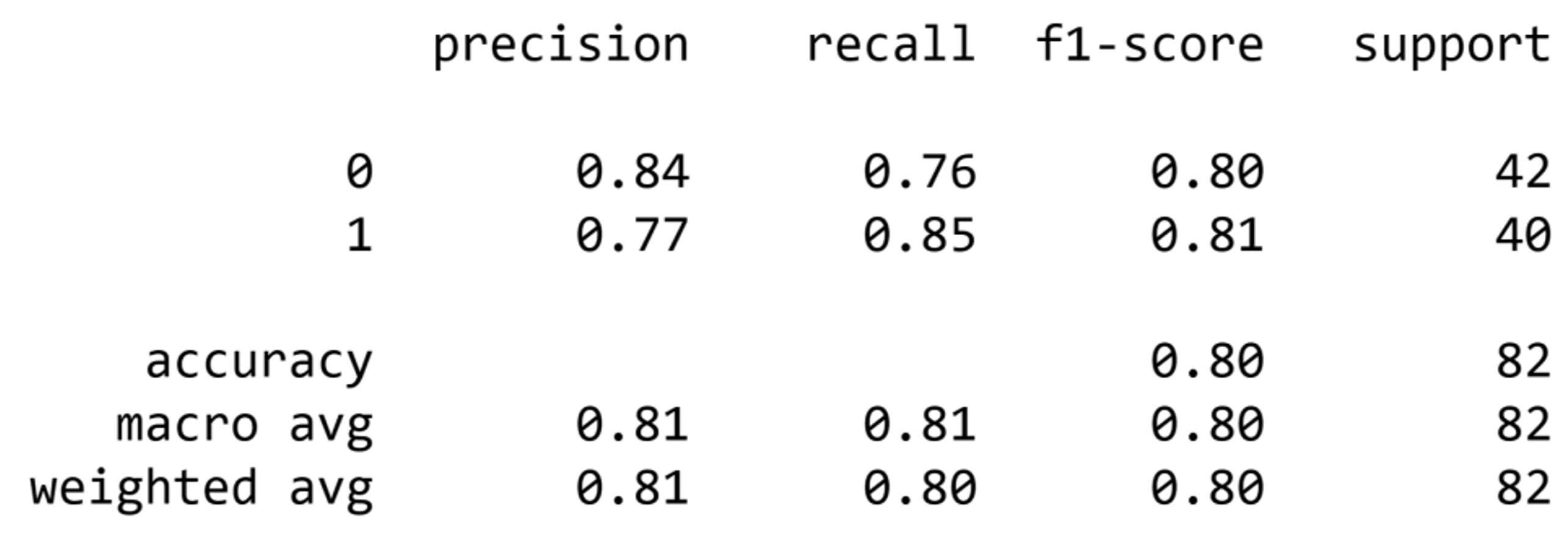
Image source: Edlitera.

As you can see, it is effortless to create a Decision Tree classifier and train it to solve classification problems. Even with a small dataset, like in the example above, I still achieved decent results using a Decision Tree model.

Decision Trees are powerful classic machine learning algorithms that can solve both classification and regression problems. Nowadays, however, Decision Trees are not used that often because more advanced algorithms supersede them. Nonetheless, knowing how Decision Trees work is crucial to understanding more complex models because more advanced algorithms, or ensemble models, are typically based on Decision Trees.

In this article, you’ve learned how a Decision Tree classifier works, how to train a Decision Tree classifier, and how to use it to make predictions. You’ve also learned how to implement one such classifier in Python to solve a binary classification problem through the example I gave. Even though the dataset was less than ideal, we achieved decent results using a Decision Tree algorithm, which shows how powerful they can be. 

 

• Read next article in the series: How to Evaluate Classification Models>>