AI models have become increasingly difficult to run on consumer-grade GPUs. As new models emerge and outperform their predecessors, they constantly require more computational power to operate efficiently. Naturally, there are exceptions. The DeepSeek model, for example, demonstrated that it is possible to compete with the most prominent models without requiring as much computational power. Even so, model size generally remains directly correlated with performance capabilities.

• DeepSeek: A Paradigm Shift in The Landscape of Large Language Models

Traditionally, deploying AI at scale meant dealing with complex infrastructure management. This overhead has become a major bottleneck for many ML teams. Members not only need to focus on improving current models but also on provisioning servers, writing deployment scripts, and managing cloud-specific services. Modal, the platform we will cover in this article, aims to address these challenges.

What Is Modal 

Modal Labs, launched in 2023, offers cloud-agnostic AI computing as a service. It is a unified cloud platform designed specifically for AI and data processing tasks. The platform enables developers to build AI workflows without requiring server configuration or managing cloud infrastructure. This allows teams to focus entirely on code and algorithms, while Modal handles the rest. Users also get easy access to a wide range of high-end GPUs, from cost-effective NVIDIA T4 models to the cutting-edge NVIDIA B200 models, which represent the crème de la crème of NVIDIA's current lineup.

• A Hands-On Guide to Experimenting with AI Agents

What sets Modal apart from other cloud platforms is its complete abstraction of infrastructure design. Developers interact with it through a Python SDK, defining "apps" and "functions" that Modal runs on demand. This approach, known as "Functions-as-a-Service", allows Python functions to execute remotely with simple decorators or API calls, similar to AWS Lambda and Google Cloud Functions. However, Modal goes further by allowing developers to declare container images and hardware directly in Python. This eliminates the need for YAML files or separate DevOps scripts.

• Building a Video Editing App in Python: How to Validate and Synchronize Text Edits with Timestamps

Unlike conventional approaches that rely on Docker or Kubernetes, Modal allows developers to specify everything in Python code. The platform uses special lightweight virtual machines managed by container engines to isolate programs from one another. More specifically, Modal leverages Google's gVisor container runtime, which provides secure isolation between the host OS and the containerized applications.

In Modal, the entire infrastructure is defined directly in Python code:

• Container
• Dependencies
• Hardware

Furthermore, users can define secrets when they need to provide an API token for a part of their code to run. They can also handle data with Modal Volumes, a built-in high-performance distributed file system that stores data and shares it between function runs. In addition, Modal supports mounting external storage, such as AWS S3 buckets, directly into functions.

How to Run Code on the Modal Platform?

The first step is to define our container and its dependencies. We do this using the Image class from Modal. This class allows us to specify the environment where our functions will run. You can think of it as similar to a Docker image. When creating an instance of the Image class, we can specify our base OS and the Python version we want to use. We can also list the Python packages to install and include any necessary system-level tools. 

• Building a Video Editing App in Python: How Do Preprocessing and Transcription Work

For example, to specify which libraries your container requires, add the following at the top of your Python script:

import modal

app = modal.App(name="example-flux-model")

image = modal.Image.debian_slim(python_version="3.10").pip_install(
    "accelerate==0.31.0",
    "transformers~=4.41.2",
    "torch~=2.2.0",
    "huggingface-hub==0.26.2",
    "numpy<2",
)

As can be seen, everything is handled in Python without the need for external files. However, before defining the image, we first need to create a Modal app, as an instance of the App class. The App object serves as the main container that groups all our functions and configurations.

You can think of an app as a deployable project running on Modal. This ensures that functions and classes maintain consistent identities across your local machine and the remote Modal containers. Apps can be ephemeral (temporary) or deployed (persistent until manually deleted). The choice depends on scaling requirements and use case objectives. Here is an example of a typical Modal script:

import modal

image = modal.Image.debian_slim().pip_install(
    "requests",
    "beautifulsoup4"
)

app = modal.App(name="my-first-app")

@app.function(image=image)
def get_page_title(url):
    """This function runs remotely, fetches a URL, and returns its title."""
    import requests
    from bs4 import BeautifulSoup

    print(f"Remotely fetching title from: {url}")

    try:
        response = requests.get(url)
        soup = BeautifulSoup(response.content, 'html.parser')
        return soup.title.string
    except Exception as e:
        return f"Could not fetch title: {e}"

@app.local_entrypoint()
def main():
    print("Fetching web page title") 
    title = get_page_title.remote("https://www.bbc.com/news") 
    print("Finished fetching title")  
    print(title)  

As can be seen in the code above, we first defined our container by creating an instance of the Image class. Then, we created an instance of the App class. This allows us to package all our code together and run it on the Modal platform. Afterward, we created a function that we want to run on Modal. It is a simple function that fetches a URL and returns its title. Finally, we defined the main function, which will execute when we run the script. If you look closely, you will notice two decorators above our functions. Each one serves a particular purpose.

• Building a Video Editing App in Python: How to Create a UI with Streamlit (Part 1)

The @app.function() decorator in Modal is a powerful tool for defining and configuring serverless functions. It accepts various arguments that let you control the execution environment, resource allocation, scheduling, and other key aspects of your function. The most important arguments are:

• image - specifies the container image used for the function's environment.
• secrets - allows you to securely pass secrets, such as API keys, to your function.
• mounts - lets you mount local files or directories into the container.
• gpu - requests Modal to run the code on a specific GPU.
• cpu - allows you to request a specific number of CPU cores for your function.
• volumes - attaches a Volume object to your function for persistent storage.

Other arguments let you control how the function executes, including concurrency and scaling options. However, the ones listed above are the most commonly used.

The @app.local_entrypoint() decorator in Modal designates a specific function as the main entry point when the script runs directly from your local command line. Unlike @app.function(), which defines functions to run remotely on Modal's infrastructure, @app.local_entrypoint() defines what happens on your local machine. You can think of it as the if __name__ == "__main__"  of Modal scripts. It serves as the starting point that orchestrates and invokes the remote functions defined with @app.function().

In addition to the decorators mentioned earlier, there is another important one that isn't shown in the code above. That is the @app.cls() decorator. It allows us to define a stateful class that runs on Modal's infrastructure. A function decorated with @app.function() is designed for a single, stateless computation that starts, runs, and terminates. A class decorated with @app.cls() initializes its state once. It can then handle multiple method calls using that persistent state.

Example: How to Train a CNN on Modal

Let's demonstrate a typical use case for Modal: training Deep Learning models. For this example, we will use a CNN to classify images from the FashionMNIST dataset. Although this is a simple problem, it is often considered a "hello world" project in Deep Learning. This makes it the perfect candidate to show how to train a Deep Learning model on Modal. The entire Python script is named modal_cnn_example.py. You can run it in the terminal using the command modal run modal_cnn_example.py. The script looks like this:

import modal
import torch
import torch.nn as nn
import torch.optim as optim
from torchvision import datasets, transforms
from torch.utils.data import DataLoader
import numpy as np
import matplotlib.pyplot as plt
from sklearn.metrics import accuracy_score, classification_report
import io
import base64

# Define Modal app and image
app = modal.App("fashion-mnist-cnn")
image = modal.Image.debian_slim().pip_install(
    "torch", "torchvision", "numpy", "scikit-learn", "matplotlib"
)


# Define CNN model
class FashionCNN(nn.Module):
    def __init__(self):
        super().__init__()
        self.conv_layers = nn.Sequential(
            nn.Conv2d(1, 32, kernel_size=3, padding=1),
            nn.ReLU(),
            nn.MaxPool2d(2),
            nn.Conv2d(32, 64, kernel_size=3, padding=1),
            nn.ReLU(),
            nn.MaxPool2d(2)
        )
        self.fc_layers = nn.Sequential(
            nn.Linear(64 * 7 * 7, 128),
            nn.ReLU(),
            nn.Linear(128, 10)
        )

    def forward(self, x):
        x = self.conv_layers(x)
        x = x.view(x.size(0), -1)
        x = self.fc_layers(x)
        return x


# Define training function with validation and testing
@app.function(image=image, gpu="any", timeout=1200)
def train_and_evaluate():
    # Set device
    device = torch.device("cuda" if torch.cuda.is_available() else "cpu")
    print(f"Using device: {device}")

    # Prepare data
    transform = transforms.Compose([
        transforms.ToTensor(),
        transforms.Normalize((0.5,), (0.5,))
    ])

    # Load datasets
    train_set = datasets.FashionMNIST(
        root="./data", train=True, download=True, transform=transform
    )
    test_set = datasets.FashionMNIST(
        root="./data", train=False, download=True, transform=transform
    )

    train_loader = DataLoader(train_set, batch_size=64, shuffle=True)
    test_loader = DataLoader(test_set, batch_size=64, shuffle=False)

    # Initialize model, loss, and optimizer
    model = FashionCNN().to(device)
    criterion = nn.CrossEntropyLoss()
    optimizer = optim.Adam(model.parameters(), lr=0.001)

    # Training loop
    model.train()
    train_losses = []
    for epoch in range(5):
        running_loss = 0.0
        for images, labels in train_loader:
            images, labels = images.to(device), labels.to(device)

            optimizer.zero_grad()
            outputs = model(images)
            loss = criterion(outputs, labels)
            loss.backward()
            optimizer.step()

            running_loss += loss.item()

        epoch_loss = running_loss / len(train_loader)
        train_losses.append(epoch_loss)
        print(f"Epoch {epoch + 1}, Loss: {epoch_loss:.4f}")

    # Save model
    torch.save(model.state_dict(), "fashion_mnist_cnn.pth")
    print("Training complete! Model saved.")

    # Validation on test set
    model.eval()
    all_preds = []
    all_labels = []

    with torch.no_grad():
        for images, labels in test_loader:
            images, labels = images.to(device), labels.to(device)
            outputs = model(images)
            _, preds = torch.max(outputs, 1)

            all_preds.extend(preds.cpu().numpy())
            all_labels.extend(labels.cpu().numpy())

    # Calculate metrics
    test_accuracy = accuracy_score(all_labels, all_preds)
    print(f"\nTest Accuracy: {test_accuracy:.4f}")

    # Classification report
    class_names = ['T-shirt/top', 'Trouser', 'Pullover', 'Dress', 'Coat',
                   'Sandal', 'Shirt', 'Sneaker', 'Bag', 'Ankle boot']
    report = classification_report(all_labels, all_preds, target_names=class_names)
    print("\nClassification Report:")
    print(report)

    # Calculate accuracy on the training set
    train_preds = []
    train_labels = []

    with torch.no_grad():
        for images, labels in train_loader:
            images, labels = images.to(device), labels.to(device)
            outputs = model(images)
            _, preds = torch.max(outputs, 1)

            train_preds.extend(preds.cpu().numpy())
            train_labels.extend(labels.cpu().numpy())

    train_accuracy = accuracy_score(train_labels, train_preds)
    print(f"\nTraining Accuracy: {train_accuracy:.4f}")

    # Inference demonstration
    print("\nRunning inference on sample test images...")
    sample_images, sample_labels = next(iter(test_loader))
    sample_images, sample_labels = sample_images.to(device), sample_labels.to(device)

    with torch.no_grad():
        sample_outputs = model(sample_images)
        _, sample_preds = torch.max(sample_outputs, 1)

    # Create visualization
    fig = plt.figure(figsize=(15, 7))
    for i in range(10):
        plt.subplot(2, 5, i + 1)
        plt.imshow(sample_images[i].cpu().squeeze(), cmap='gray')
        plt.title(f"True: {class_names[sample_labels[i]]}\nPred: {class_names[sample_preds[i]]}")
        plt.axis('off')

    plt.tight_layout()

    # Save plot to buffer
    buf = io.BytesIO()
    plt.savefig(buf, format='png')
    buf.seek(0)
    img_base64 = base64.b64encode(buf.read()).decode('utf-8')
    plt.close()

    # Return results
    return {
        "train_accuracy": float(train_accuracy),
        "test_accuracy": float(test_accuracy),
        "classification_report": report,
        "sample_predictions": img_base64
    }


# Entry point
@app.local_entrypoint()
def main():
    results = train_and_evaluate.remote()

    print("\n=== FINAL RESULTS ===")
    print(f"Training Accuracy: {results['train_accuracy']:.4f}")
    print(f"Test Accuracy: {results['test_accuracy']:.4f}")
    print("\nClassification Report:")
    print(results['classification_report'])

    # Save sample predictions image
    img_data = base64.b64decode(results['sample_predictions'])
    with open("sample_predictions.png", "wb") as f:
        f.write(img_data)
    print("\nSample predictions saved to 'sample_predictions.png'")

Let's break down this code.

How to Import Dependencies

The first step is to import the necessary dependencies.

import modal
import torch
import torch.nn as nn
import torch.optim as optim
from torchvision import datasets, transforms
from torch.utils.data import DataLoader
import numpy as np
import matplotlib.pyplot as plt
from sklearn.metrics import accuracy_score, classification_report
import io
import base64

Each of these imported libraries serves a specific purpose:

• modal - enables serverless execution on Modal's platform.
• torch and related modules - used for building and training the neural network.
• torchvision - provides access to the FashionMNIST dataset.
• numpy - supports numerical operations.
• matplotlib is used for visualizing results.
• sklearn.metrics - helps evaluate model performance.
• io and base64 - handle image outputs.

After importing the dependencies, we can move on to the next step.

How to Configure a Modal App

In this step, we create a new Modal application and give it an appropriate name, in this case "fashion-mnist-cnn". Next, we define our image with all the required dependencies. The image uses a lightweight Linux base, and all necessary libraries are installed inside it using pip.

# Define Modal app and image
app = modal.App("fashion-mnist-cnn")
image = modal.Image.debian_slim().pip_install(
    "torch", "torchvision", "numpy", "scikit-learn", "matplotlib"
)

Once the application is created and the image is defined, we can move on to creating the model.

How to Define the CNN Model Architecture

Now, we will define the architecture of our CNN model. In practice, we set up everything locally and delegate the "heavy lifting" to Modal. 

# Define CNN model
class FashionCNN(nn.Module):
    def __init__(self):
        super().__init__()
        self.conv_layers = nn.Sequential(
            nn.Conv2d(1, 32, kernel_size=3, padding=1),
            nn.ReLU(),
            nn.MaxPool2d(2),
            nn.Conv2d(32, 64, kernel_size=3, padding=1),
            nn.ReLU(),
            nn.MaxPool2d(2)
        )
        self.fc_layers = nn.Sequential(
            nn.Linear(64 * 7 * 7, 128),
            nn.ReLU(),
            nn.Linear(128, 10)
        )
    def forward(self, x):
        x = self.conv_layers(x)
        x = x.view(x.size(0), -1)
        x = self.fc_layers(x)
        return x

The code above defines a simple CNN architecture with two convolutional blocks. Each block contains convolutional layers with ReLU activation and max pooling. The network takes a grayscale image of size 28x28 from the FashionMNIST dataset as input. It then passes the image through the convolutional blocks and fully connected layers, producing a final prediction. This prediction assigns the image to one of ten possible classes.

• Intro to Image Augmentation: What Are Pixel-Based Transformations?

After defining the model architecture, we can proceed to define the training and evaluation functions.

How to Define the Main Training and Evaluation Function

Since this function is fairly complex, let's break it down into smaller segments.

Part 1: How to Decorate the Function

At the very top, right above the function, we need to add a decorator that ensures it runs on the Modal platform.

@app.function(image=image, gpu="any", timeout=1200)

This line of code ensures that Modal uses the image we defined earlier, runs the code on a GPU, and sets a 20-minute timeout for the function. If you want to target a specific GPU, you can set the value of the gpu argument to the desired model, such as "H100", instead of "any".

Part 2: How to Set Up the Device

Simply specifying a GPU in the decorator is not enough. We also need to set up our model to use the GPU for training. This can be done with the following line of code:

# Set device
device = torch.device("cuda" if torch.cuda.is_available() else "cpu")
print(f"Using device: {device}")

The code above attempts to detect a GPU. If one is available, it moves the model to that device. A print statement was also included to confirm whether the model was successfully moved to the GPU provided by Modal. 

Part 3: How to Prepare Data

In this part of the code, we first define our data preprocessing pipeline. This includes the following:

• The transformation pipeline
• Constructing datasets
• Constructing dataloaders

# Prepare data
transform = transforms.Compose([
    transforms.ToTensor(),
    transforms.Normalize((0.5,), (0.5,))
])

# Load datasets
train_set = datasets.FashionMNIST(
    root="./data", train=True, download=True, transform=transform
)
test_set = datasets.FashionMNIST(
    root="./data", train=False, download=True, transform=transform
)

train_loader = DataLoader(train_set, batch_size=64, shuffle=True)
test_loader = DataLoader(test_set, batch_size=64, shuffle=False)

The transformation pipeline converts images to PyTorch tensors and normalizes pixel values by mapping them into a certain range. This pipeline is applied when constructing our datasets, which we create by downloading the FashionMNIST data directly from the datasets module of the torchvision library. Finally, we create data loaders that feed data to the model in batches of 64 samples.

Part 4: How to Initialize the Model 

After completing the data preprocessing pipeline, we can initialize our model and define the loss function and optimizer for training.

# Initialize model, loss, and optimizer
model = FashionCNN().to(device)
criterion = nn.CrossEntropyLoss()
optimizer = optim.Adam(model.parameters(), lr=0.001)

Since this is a multiclass classification problem, we will use the cross-entropy loss function. For optimization, we will use Adam, one of the most popular Deep Learning optimizers, with a starting learning rate of 0.001.

Part 5: How to Train and Evaluate the Model

The next step is to define the training and evaluation loops. Let's start with the training loop:

# Training loop
model.train()
train_losses = []
for epoch in range(5):
    running_loss = 0.0
    for images, labels in train_loader:
        images, labels = images.to(device), labels.to(device)

        optimizer.zero_grad()
        outputs = model(images)
        loss = criterion(outputs, labels)
        loss.backward()
        optimizer.step()

        running_loss += loss.item()

    epoch_loss = running_loss / len(train_loader)
    train_losses.append(epoch_loss)
    print(f"Epoch {epoch + 1}, Loss: {epoch_loss:.4f}")

In this loop, we set the model to training mode and run training for 5 epochs. Within each epoch, every batch is processed in the following way:

• The data is moved to the appropriate device.
• Previous gradients are cleared.
• A forward pass is performed to generate model predictions.
• The loss is calculated.
• A backward pass computes the gradients.
• The model parameters are updated.

We will also track and print the average loss for each epoch. Finally, we save the  trained model using the following code:

# Save model
torch.save(model.state_dict(), "fashion_mnist_cnn.pth")
print("Training complete! Model saved.")

The next step is to define the validation loop, which will validate our model's performance on the test set:

# Validation on test set
model.eval()
all_preds = []
all_labels = []

with torch.no_grad():
    for images, labels in test_loader:
        images, labels = images.to(device), labels.to(device)
        outputs = model(images)
        _, preds = torch.max(outputs, 1)

        all_preds.extend(preds.cpu().numpy())
        all_labels.extend(labels.cpu().numpy())

# Calculate metrics
test_accuracy = accuracy_score(all_labels, all_preds)
print(f"\nTest Accuracy: {test_accuracy:.4f}")

# Classification report
class_names = ['T-shirt/top', 'Trouser', 'Pullover', 'Dress', 'Coat',
               'Sandal', 'Shirt', 'Sneaker', 'Bag', 'Ankle boot']
report = classification_report(all_labels, all_preds, target_names=class_names)
print("\nClassification Report:")
print(report)

In the validation loop, we do the following:

• Set the model to evaluation mode.
• Disable gradient computation to improve efficiency.
• Generate predictions on the test set.
• Calculate the model's accuracy and produce a classification report.

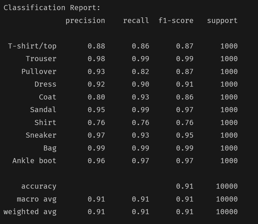
The classification report we generate at the end provides valuable insights into our model's performance. It includes detailed metrics such as precision, recall, and the F1 score for each class.

• The Model Context Protocol (MCP): A Universal Standard for AI Agent Integration

Here, I also decided to evaluate the model on the training set. Specifically, I print the accuracy achieved on the training set so we can compare it to the accuracy achieved on the test set. This comparison helps us determine whether the model is overfitting or underfitting:

# Calculate accuracy on the training set 
train_preds = []
train_labels = []

with torch.no_grad():
    for images, labels in train_loader:
        images, labels = images.to(device), labels.to(device)
        outputs = model(images)
        _, preds = torch.max(outputs, 1)

        train_preds.extend(preds.cpu().numpy())
        train_labels.extend(labels.cpu().numpy())

train_accuracy = accuracy_score(train_labels, train_preds)
print(f"\nTraining Accuracy: {train_accuracy:.4f}")

In my case, when running the code, I get the following results:

• A training accuracy of 0.9438
• A test accuracy of 0.9138

This outcome is expected. When a model is neither overfitting nor underfitting, the accuracy on the test set is typically slightly lower than that on the training set. If we had trained the model for more than five epochs, the results would likely have improved. The classification report I obtained is as follows:

As can be seen, our model performs better at predicting certain classes than others. However, training the model for more epochs would likely improve this imbalance.

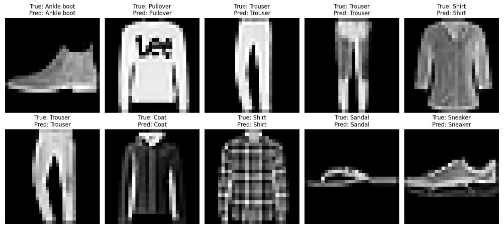
Part 6: How to Perform Inference

Training and evaluating the model is important to understand its performance. However, ultimately, we train models to use them in production, which means to perform inference. We can do this using the following code:

# Inference demonstration
print("\nRunning inference on sample test images...")
sample_images, sample_labels = next(iter(test_loader))
sample_images, sample_labels = sample_images.to(device), sample_labels.to(device)

with torch.no_grad():
    sample_outputs = model(sample_images)
    _, sample_preds = torch.max(sample_outputs, 1)


# Create visualization
fig = plt.figure(figsize=(15, 7))
for i in range(10):
    plt.subplot(2, 5, i + 1)
    plt.imshow(sample_images[i].cpu().squeeze(), cmap='gray')
    plt.title(f"True: {class_names[sample_labels[i]]}\nPred: {class_names[sample_preds[i]]}")
    plt.axis('off')

plt.tight_layout()

# Save plot to buffer
buf = io.BytesIO()
plt.savefig(buf, format='png')
buf.seek(0)
img_base64 = base64.b64encode(buf.read()).decode('utf-8')
plt.close()

In the code above, we perform the following steps:

• Run inference on a sample batch from the test set.
• Create a plot using matplotlib.
• Convert the plot to a base64-encoded string for easy transfer.

The visualization we create displays the first 10 images in a batch, along with their true labels and the model's predictions. In my case, it looks like this:

The final block of code, at the very end, is where we package all the results into a dictionary:

# Return results
return {
    "train_accuracy": float(train_accuracy),
    "test_accuracy": float(test_accuracy),
    "classification_report": report,
    "sample_predictions": img_base64
}

As can be seen, the dictionary includes the calculated accuracies, the classification report, and the results from the inference.

How to Define the Entry Point

At the end of the script, after defining the main training and evaluation function, we define the entry point for local execution:

# Entry point
@app.local_entrypoint()
def main():
    results = train_and_evaluate.remote()

    print("\n=== FINAL RESULTS ===")
    print(f"Training Accuracy: {results['train_accuracy']:.4f}")
    print(f"Test Accuracy: {results['test_accuracy']:.4f}")
    print("\nClassification Report:")
    print(results['classification_report'])

    # Save sample predictions image
    img_data = base64.b64decode(results['sample_predictions'])
    with open("sample_predictions.png", "wb") as f:
        f.write(img_data)
    print("\nSample predictions saved to 'sample_predictions.png'")

The code above performs the following actions:

• Defines the entry point for local execution using the decorator.
• Calls the remote function on Modal.
• Prints the result.
• Decodes and saves the plot we created as a PNG file

Modal simplifies AI development by eliminating the hassle of managing servers and cloud infrastructure. Instead of dealing with these complexities, developers can focus on what they do best: building and improving their models.

• Absolute Zero: How AI Learns to Reason Without Human Data

As demonstrated in the FashionMNIST example, Modal enables users to train models on powerful GPUs using just a few lines of Python code. There is no need to set up servers, write complex deployment scripts, or manage cloud configurations.

For teams aiming to accelerate their AI projects without the usual technical overhead, Modal provides a simple solution. It makes serverless computing accessible and efficient for AI developers.