


Table of Contents
While some would call it easy compared to some of the more complex services on Amazon's cloud platform, AWS Glue still requires certain prerequisite knowledge. You need to be familiar with a few key data engineering concepts to understand the benefits of using Glue. Some examples of these concepts are what data engineering is, the difference between a data warehouse and a data lake, as well as ETL and ELT, and a few other concepts.
In this article, I will first cover these topics. Then, I will shift the focus to AWS Glue and AWS Glue DataBrew and what they offer. After explaining the theory behind Glue and DataBrew, I will dive deep into an example, in which I will demonstrate how to use Glue DataBrew to create a data workflow.
What is Data Engineering?
Every data scientist understands the importance of data engineering. However, most people tend to find it less interesting and try to rush through it or ignore it. This is a consequence of the popularity of AI. Most people getting into the fields of machine learning and deep learning focus on creating models that give great predictions using collected data. Those same people may not realize the implications of not having quality data at their disposal. Even the most revolutionary model won't get good results if the data it trains on is subpar.
Without an investment in data engineering, an organization will only ever use a fraction of all the data available. As technology advanced, an ever-increasing number of data sources was made available. These large quantities of data are knows as big data. Data engineering focuses on creating efficient ways of collecting these huge quantities of data and analyzing it.
To be more specific, data engineers don't focus as much on experimental design, but instead focus on creating mechanisms that regulate data flow and allow for quick and easy data retrieval. The job of a data engineer is a very demanding one because it requires detailed knowledge and understanding of many topics, including:
- Data models
- Information flow
- Query execution and optimization
- Design of relational and non-relational databases
- ETL
With the introduction and rise in popularity of cloud platforms, being a data engineer today requires knowing more tools than ever before, such as Spark, Hive, and Hadoop. Though this is the case nowadays, there is a chance that almost all companies will use cloud platforms in the near future. Even though this won't decrease the amount of knowledge a data engineer needs to have, it might lead to a situation where data engineers can focus on a cloud platform of their choice and become specialized in it, in effect reducing the number of different tools they need to know.
What is a Data Warehouse?
Often called decision support databases, data warehouses are separate from an organization's operational database. They are the core of an organization’s business intelligence system. You access data that is stored in a data warehouse using various business intelligence tools, SQL clients, and spreadsheets.
Data warehouses are created so that you can easily query and analyze data collected from many different sources. This also makes data mining efficient and possible.
The four main components of a data warehouse are:
- Load Manager - the front component, in charge of data extraction and loading
- Warehouse Manager - in charge of performing data analysis, creating indexes and views, data merging, data aggregation, etc.
- Query Manager - the back component, manages user queries
- End-User Access Tools - query tools, tools that create data reports, application development tools, data mining tools, EIS tools, and OLAP tools
What Are the Advantages of a Data Warehouse?
- Highly scalable and good for big data
- Increase speed and efficiency of data analytics
- Give a combined view of data, allowing users to create good reports
- Perfect for analyzing different time periods to predict future trends
What Are the Disadvantages of a Data Warehouse?
- Not good for unstructured data
- Too complex for the average user
- Can get outdated quickly
- Can be time-consuming to implement
What is a Data Lake?
Up until now, whenever I talked about ETL and data engineering, I talked about data warehouses. However, with cloud platforms, a new way of storing big data was introduced: data lakes.
Data lakes are repositories that can hold huge quantities of raw data. That data is stored in its raw format until it is needed. Every element in the data lake is given a unique identifier, accompanied by corresponding metadata tags. The target audience for data lakes is data scientists. Data lakes are best suited for use in data science research and testing. Contrary to data warehouses, they encourage a schema-on-read process model. Data stored in native format is retrieved dynamically when there is a need for it.
Data lakes are not designed with ETL processes in mind. Contrary to data warehouses, because they can contain structured, semi-structured, and even unstructured data, the process you use when working with data lakes is an alternative to the standard ETL process. Data lakes use the ELT process.
What Are the Advantages of Data Lakes?
- Perfectly suited to cloud computing
- They retain all data unlike data warehouses, where only some data enters the data warehouse
- They support data sources that data warehouses don't, such as sensor data, web server logs, etc., and support users that need to heavily change and manipulate data
- They adapt to change very quickly
- Data from data lakes can be accessed much quicker
What Are Disadvantages of Data Lakes?
- They assume a certain amount of user knowledge
- Sometimes they contain subpar data
- Lack of insight from previous findings
- Data integrity loss
What is ETL?
ETL is an abbreviation which you use to describe a data integration process that consists of the following three steps:
- Extract
- Transform
- Load
The main idea behind ETL processes is to create some type of construct that allows you to view data from multiple different sources. Typically, you would first create a data warehouse, then you can analyze the data in the data warehouse and create different reports. This has proven to be exceptionally practical for establishing good communication between coworkers who may have different skill levels in programming, data engineering, and data science.
Article continues below
Want to learn more? Check out some of our courses:
Extract
The first step of an ETL process is to extract data. The goal of this step is to move data from multiple different data sources to a staging area. The data can be extracted from not only homogeneous sources, but also heterogeneous sources (which is far more common).
Frequently used data source formats are:
- Relational Databases
- XML
- JSON
- Flat Files
- IMS
- VSAM
- ISAM
This is potentially the most important step of ETL since it prepares data for the next two steps. Generally, I prefer my data to be in a single format before I start the processes of transformation and loading.
Another important part of data loading is the process of data validation. The validity of the extracted data must be confirmed so that no problematic data enters the next stage of the ETL process. Data engineers should also make sure that the invalid data gets reported so that its source gets investigated, and any problems that occurred during data extraction get solved.
Transform
During this stage, you transform your data and prepare it for the next step: loading. Transformations are functions that you use to define data transformation processes. They are necessary because your data is often in need of cleaning, even if it is all in one format. I usually prefer to modify my data in some way before I load it into my end target.
That process, also called cleansing, includes procedures such as:
- Filtering
- Encoding and character set conversion
- Conversion of units of measurement
- Validating data thresholds
- Transposing rows or columns
- Merging data
- Data flow validation
There are a lot more procedures than the ones I mentioned above. The amount of transformations needed depends on the data that is extracted and enters the staging area. Cleaner data will require fewer transformations. Since this step is directly influenced by the first step in the process, changes in the first step will likely lead to changes in the second step, such as removing some transformations or adding new ones.
Load
Load is the last step of the ETL process. It covers moving transformed data from the staging area to your data warehouse. Although this process might seem very simple, the complexity of it lies in the sheer amount of data that needs to be loaded as quickly as possible.
Loading huge amounts of data quickly requires a highly optimized process, with some safety mechanisms put in place to activate in case of a load failure. There are different types of loading:
- Initial Load - populating all warehouse tables
- Incremental Load - applying periodical changes
- Full Refresh - replacing old content with fresh content
What is ELT?
As an alternative to the ETL data integration process, it functions by replacing the order of the second and third steps of the ETL process.
The steps of the ELT process are as follows:
- Extract
- Load
- Transform
Using the built-in processing capability of some data storage infrastructure, processes become much more efficient. Because the data doesn't go through an intermediary step where it gets transformed, the time that passes from extracting data to loading that data into target storage such as a data warehouse is a lot shorter.
What Are the Advantages of ELT?
- Better suited towards cloud computing and data lakes
- Data loading to the target system is significantly quicker
- Transformations performed per request which reduces the wait times for data transformation
What Are the Disadvantages ELT?
- Tools are harder to use
- ELT maintenance is virtually non-existent when compared to ETL systems
What is AWS Glue?
Glue was originally released in August 2017. Since then, it has seen many updates, the last one being in December 2020. The purpose of Glue is to allow you to easily discover, prepare, and combine data. Creating a workflow that efficiently achieves these processes can take quite some time. This is where Glue steps in. It is a fully managed ETL service specifically designed to handle large amounts of data. Its job is to extract data from several other AWS services and incorporate that data into data lakes and data warehouses.
Glue is very flexible and easy to use because it provides both code-based and visual interfaces. A very popular and recent addition is DataBrew. Using Glue, DataBrew data can be cleaned, normalized, and even enriched, without even writing code. While Glue Elastic Views makes combining and replicating data across different data stores using SQL very straightforward.
Glue jobs can be triggered by predetermined events, or can be set to activate following some schedule. Triggering a job automatically starts the ETL process. Glue will extract data, transform it using automatically generated code and load it into a data lake such as the AWS S3 service, or a data warehouse such as the Amazon Redshift service. Of course, Glue supports much more. It also supports MySQL, Oracle, Microsoft SQL Server, and PostgreSQL databases that run on EC2 instances.
All data gets profiled in the Glue Data Catalog. Customizable crawlers scan raw data stores and extract attributes from them. Data Catalog is a metadata repository that contains metadata for all data assets. It can also replace Apache Hive Metastore for Amazon Elastic MapReduce.
It should be noted that it is also possible to create and use developer endpoints. Using those endpoints, Glue can easily be debugged and custom libraries and code can be implemented, such as readers, writers.
What Are the Advantages of AWS Glue?
- Easy maintenance and deployment
- Cost-efficient
- Easy to debug
- Supports many different data sources
What Are the Disadvantages of AWS Glue?
- Not the best for real-time ETL
- Limited compatibility with non-AWS services
- Limited support for queries
What is AWS Glue DataBrew?
DataBrew is a relatively new addition to the AWS family of services, introduced in November of 2020. It is a visual data preparation tool that requires no coding whatsoever, which means it is very accessible even for those who may not be adept at programming. Because the tool requires no coding at all (and because of how DataBrew recipes work, which is something I will explain later on in this article), the tool makes collaboration between teams inside a company very straightforward.
Inside each company, multiple teams work with data, with each team using that data differently. Data scientists, data engineers, business analysts, etc., all analyze data regularly, but the differences between those teams can sometimes lead to problems. It can be hard to communicate ideas and discuss problems between teams that are at a different level of technical knowledge.
To alleviate that problem and streamline communication between teams, AWS introduced DataBrew. They claim that it helps reduce the time needed to prepare data for analytics and machine learning by up to 80%. Leveraging the power of over 250 built-in transformations automates work to save a lot of time.
DataBrew integrates extremely well with other AWS services. When creating new projects, you can import your data from numerous different data sources such as S3 buckets, Amazon RDS tables, Amazon Redshift, etc. Also, you can profile your data, allowing you to gain an insight into it before you even start applying transformations to it. Information such as data type, level of cardinality, top unique values, whether there is missing data or not, and even how the distribution of data looks, can sometimes be crucial to determining how to deal with some data.
That being said, the fact that the current capabilities of the profiling tool inside of the service might look somewhat limited from the perspective of an advanced user is a design choice. DataBrew is not primarily a data analysis tool, so it isn't surprising that its data profiling capabilities are a bit on the light side. For a tool like DataBrew, it is far more important to have a function that tracks data lineage. In DataBrew, it comes in the form of a visual interface, which further emphasizes the idea that DataBrew should be as easy to use as possible.
However, the true power of this new AWS service lies in its ability to apply over 250 different in-built transformations without any coding. Transforming data can sometimes be code-heavy, so having the ability to perform them by just clicking a few buttons in a UI cannot be overstated. Transforming data in DataBrew is very straightforward and is contained in so-called DataBrew recipes.
What Are DataBrew Recipes?
Recipes define the flow of transformations in DataBrew. Every transformation project in DataBrew will consist of several steps. Recipes contain those steps strung together into a coherent workflow that is reusable and shareable.
As mentioned before, there are a plethora of different transformations that can be applied to data, some of which are:
- Filtering and modifying columns
- Formatting data
- Dealing with missing values
- Dealing with duplicate values
- Mathematical functions
- Creating pivot tables
- Aggregating data
- Tokenization
- Encoding data
- Scaling data
These are just some of the many functions of DataBrew. With such a vast number of different transformations at your disposal. The only thing you need to do when transforming your data is to choose the right one.
For some, it might seem like a problematic task given the sheer number of options. However, the creators of DataBrew also decided to include a recommendations tab. In this tab, you can see what transformations DataBrew recommends for a particular dataset. This further emphasizes the main idea of DataBrew: simplicity.
Glue DataBrew VS. SageMaker DataWrangler
With both services coming out in a relatively close time frame, and both serving a similar purpose, a lot of data scientists were left with a dilemma: use Glue DataBrew or SageMaker DataWrangler for dealing with data?
This question doesn't have a right answer, as it depends on your needs. Advanced users, especially data scientists, will surely mention that, in DataWrangler, you can write custom transformations on the spot and use them to transform your data. It also has the capability of quickly analyzing data on a high-level, including building quick machine learning models to track information such as feature importance.
On the other hand, the simplicity of DataBrew cannot be ignored. With as many built-in transformations as there are available in it, you might have all your needs covered. Also, working in DataBrew requires a lot less knowledge and can be used by anyone with minimal technical knowledge.
All in all, the target groups of these two services are different. DataWrangler is aimed at data scientists, focusing on giving you the freedom you need when preparing data for machine learning models. Conversely, DataBrew makes sure that things stay as simple as possible. It offers less freedom but in return covers almost everything an average user could ever want. Advanced users might find its capabilities somewhat limited, but they are not the target audience for the service.
An Example of How to Use AWS Glue DataBrew
Knowing the theory behind a service is important, but one should not neglect the importance of hands-on experience. To finish this article, I'm going to demonstrate how DataBrew works by loading in a simple dataset, profiling that dataset, and creating a DataBrew recipe.
The dataset I'm going to use is the Wine Reviews dataset found on Kaggle, specifically the winemag-data-130k-v2.csv file.
How to Create a Source of Data
This example includes a step that isn't directly connected to DataBrew, and that is creating an S3 bucket.
To create an S3 bucket, go to the S3 Management Console in AWS and click on Create bucket:
Image Source: Screenshot of AWS DataBrew S3 Bucket, Edlitera
Create a new bucket and name it edlitera-databrew-bucket.
Leave all other options on default:
Image Source: Screenshot of S3 bucket creation using AWS DataBrew, Edlitera
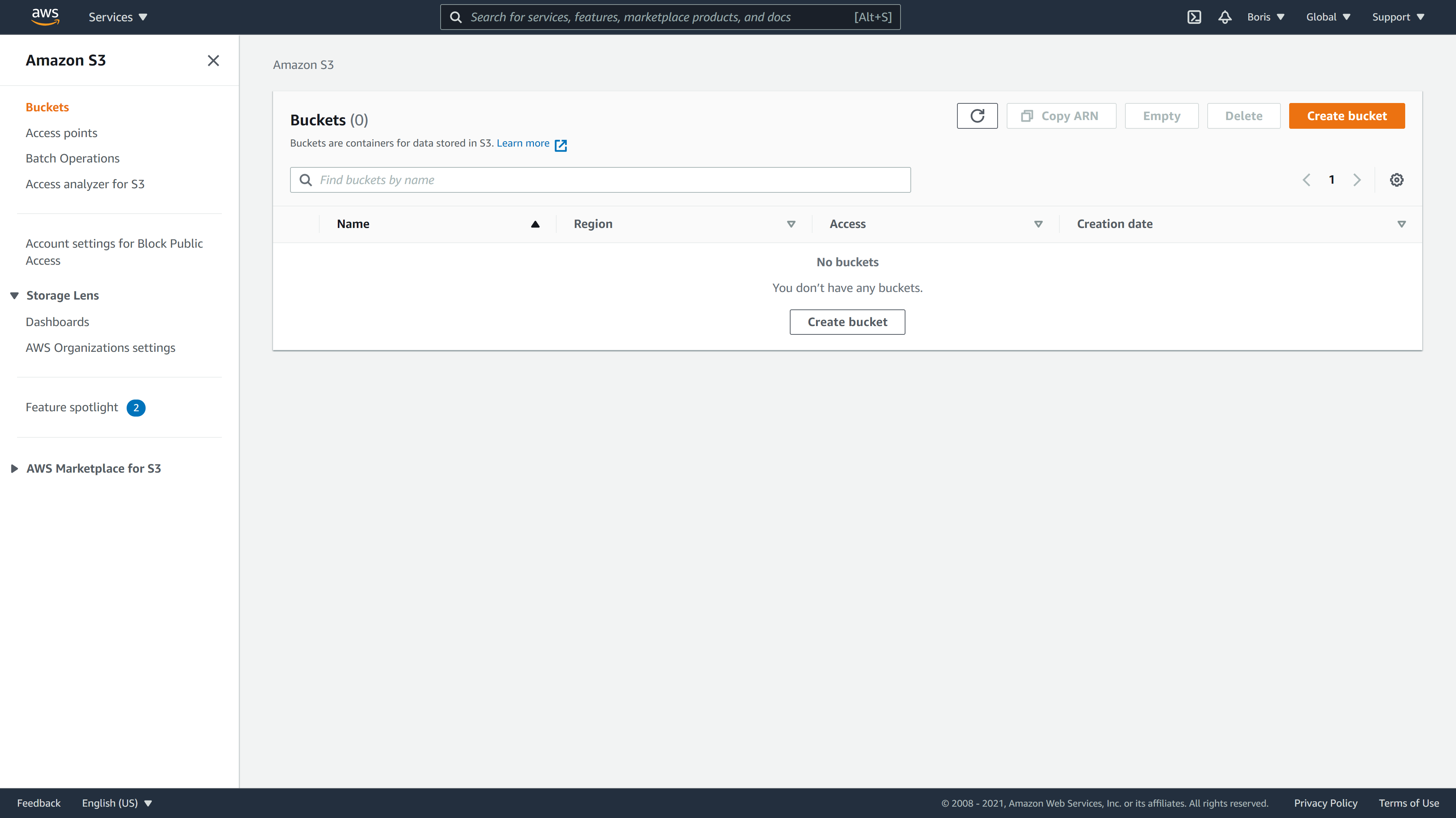
Once you create the bucket, it will pop-up on your S3 screen in AWS:
Image Source: Screenshot of AWS DataBrew, Edlitera
After creating a bucket, you are ready to start working with DataBrew.
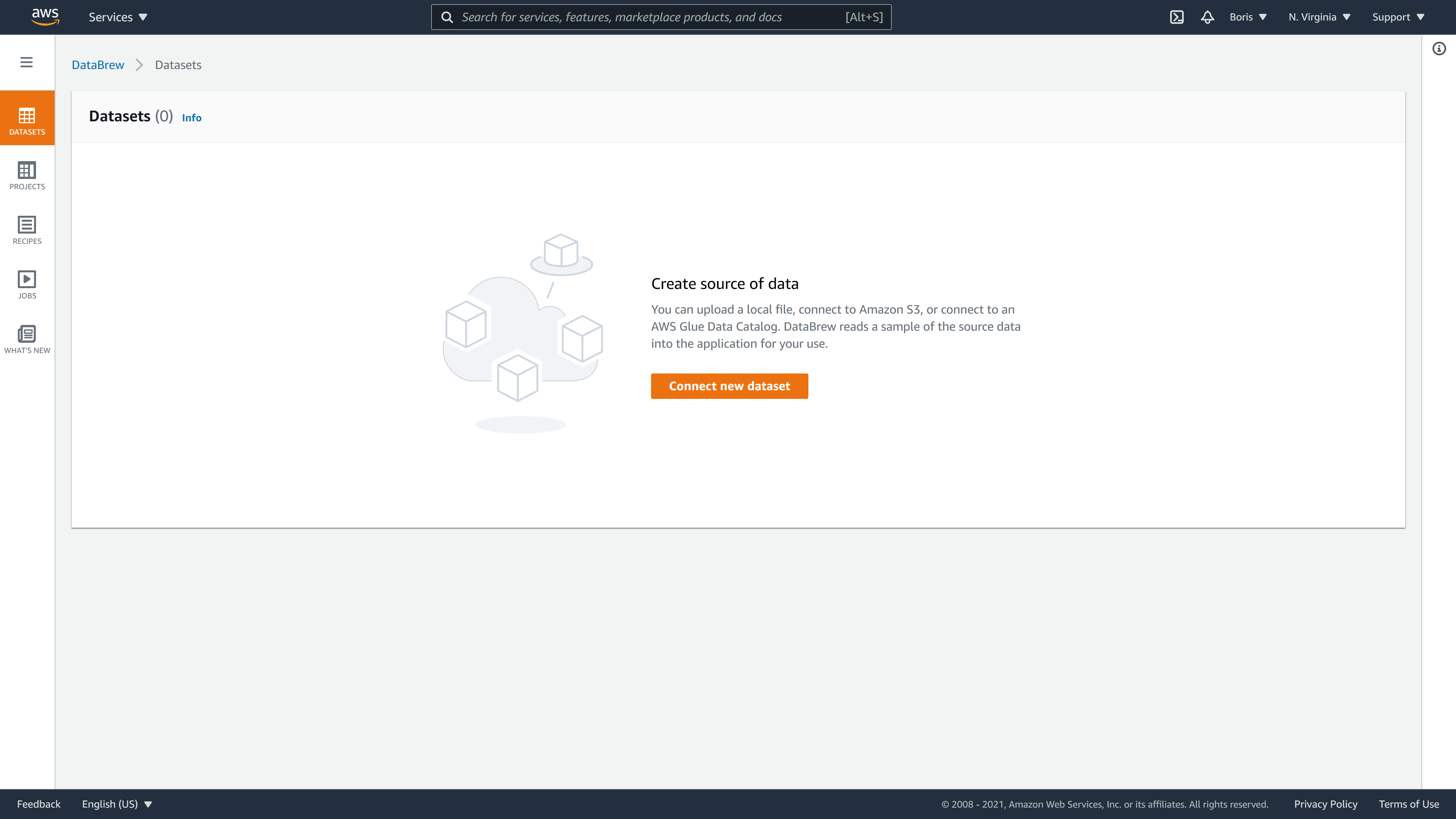
On the DataBrew page, click on the datasets tab, and afterward on Connect new dataset:
Image Source: Screenshot of AWS DataBrew, Edlitera
When connecting a new dataset, you'll need to define a few things:
- Dataset name
- Dataset source
- Output destination
- Tags (optional)
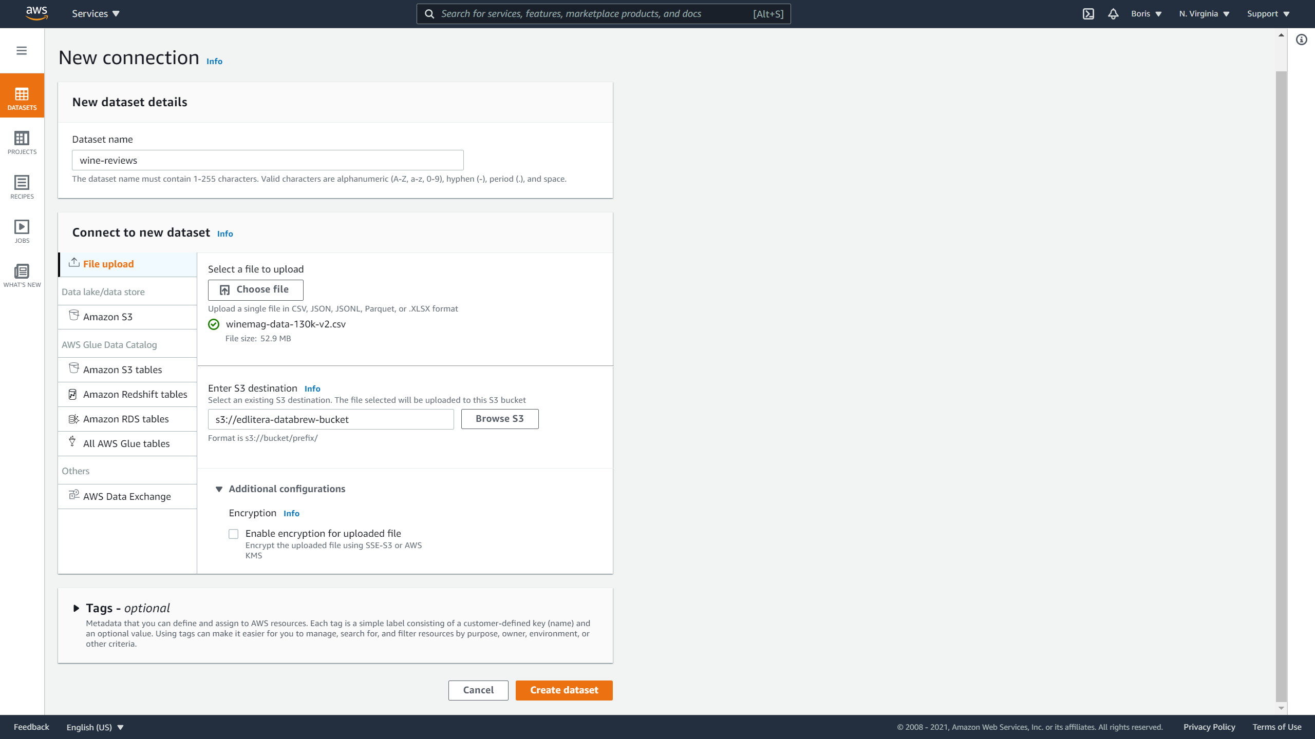
I am going to name this dataset wine-reviews and select File upload.
With file upload, you can select the dataset that you have on your local machine and tell DataBrew to upload it to the empty bucket you created earlier:
Image Source: Screenshot of AWS DataBrew, Edlitera
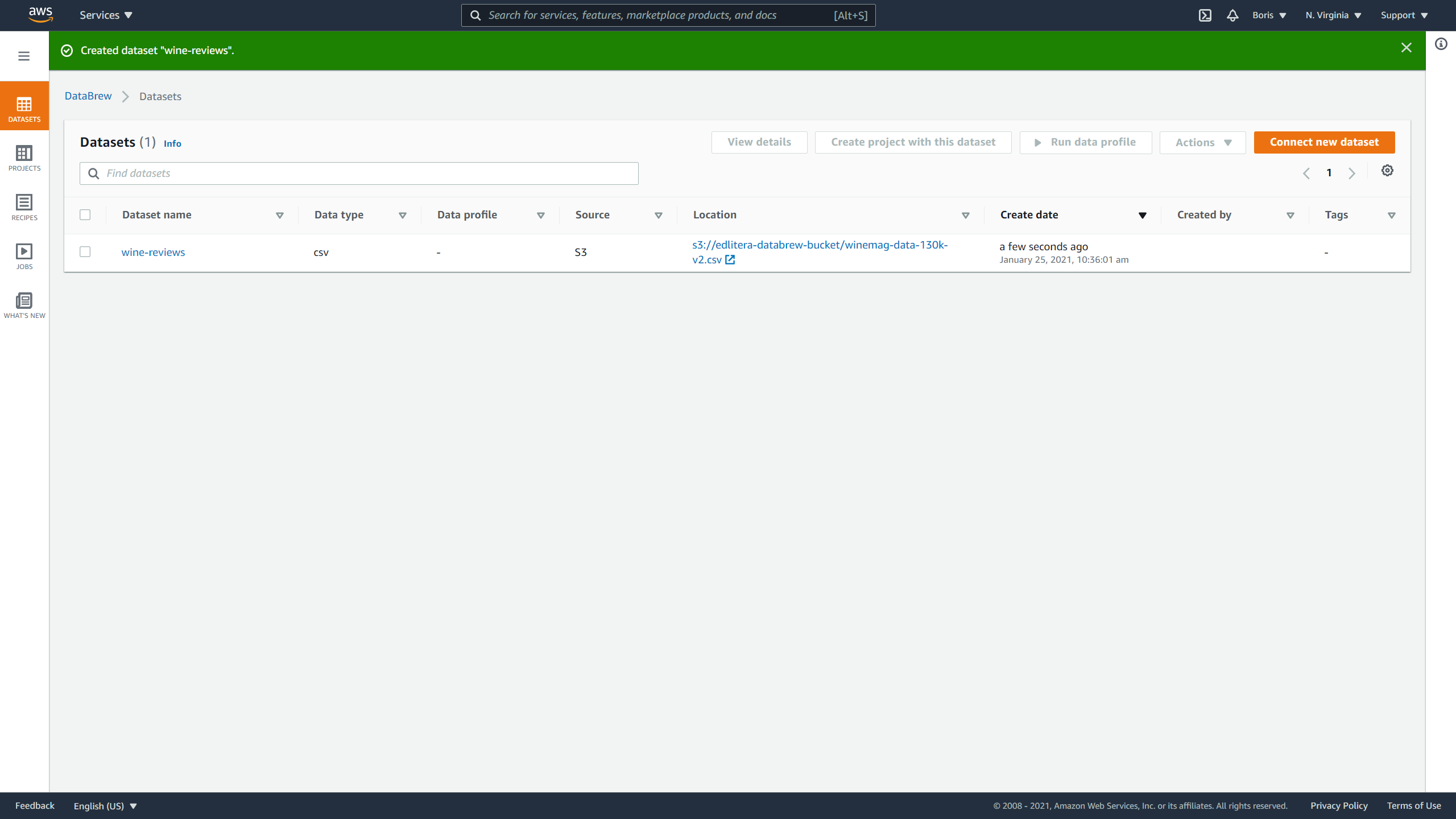
The new dataset should now be available for use.
Image Source: Screenshot of AWS DataBrew, Edlitera
How to Profile Your Data
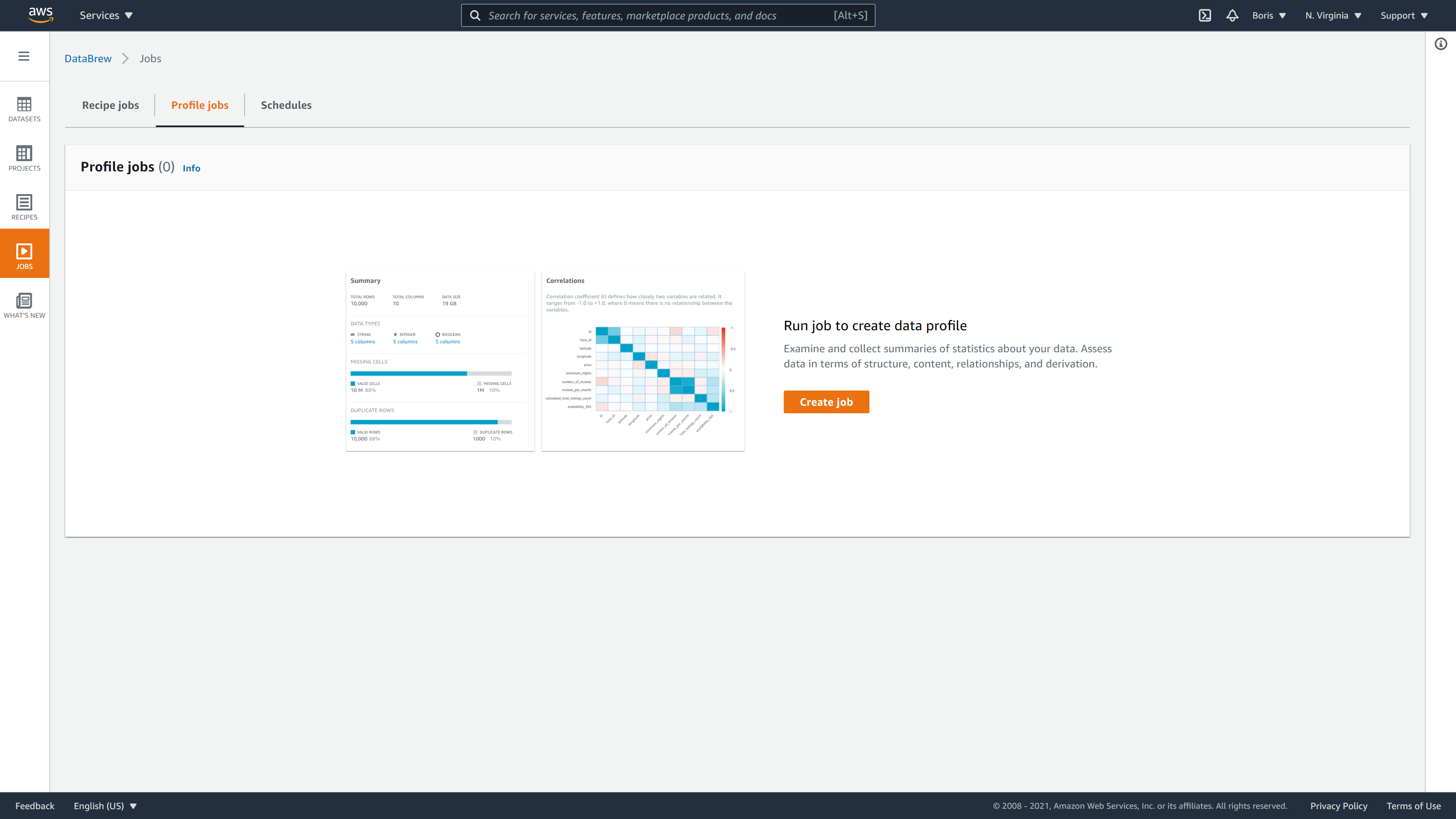
After defining the dataset you're going to use, you can do some basic data analysis. DataBrew contains a dataset profiling feature. Profiling data can be very useful when the data you are working with is unfamiliar to you. To create a profile job, you will click on the Jobs tab.
You will be offered three options:
- Recipe jobs
- Profile jobs
- Schedules
At this moment, you want to create a profile of your dataset to gain some insight into how your data looks.
Let's select the Profile jobs tab and click on Create job:
When defining the job, you will have to input values for the following parameters:
- Job name
- Job type
- Job input
- Job output settings
- Permissions
- Optional settings
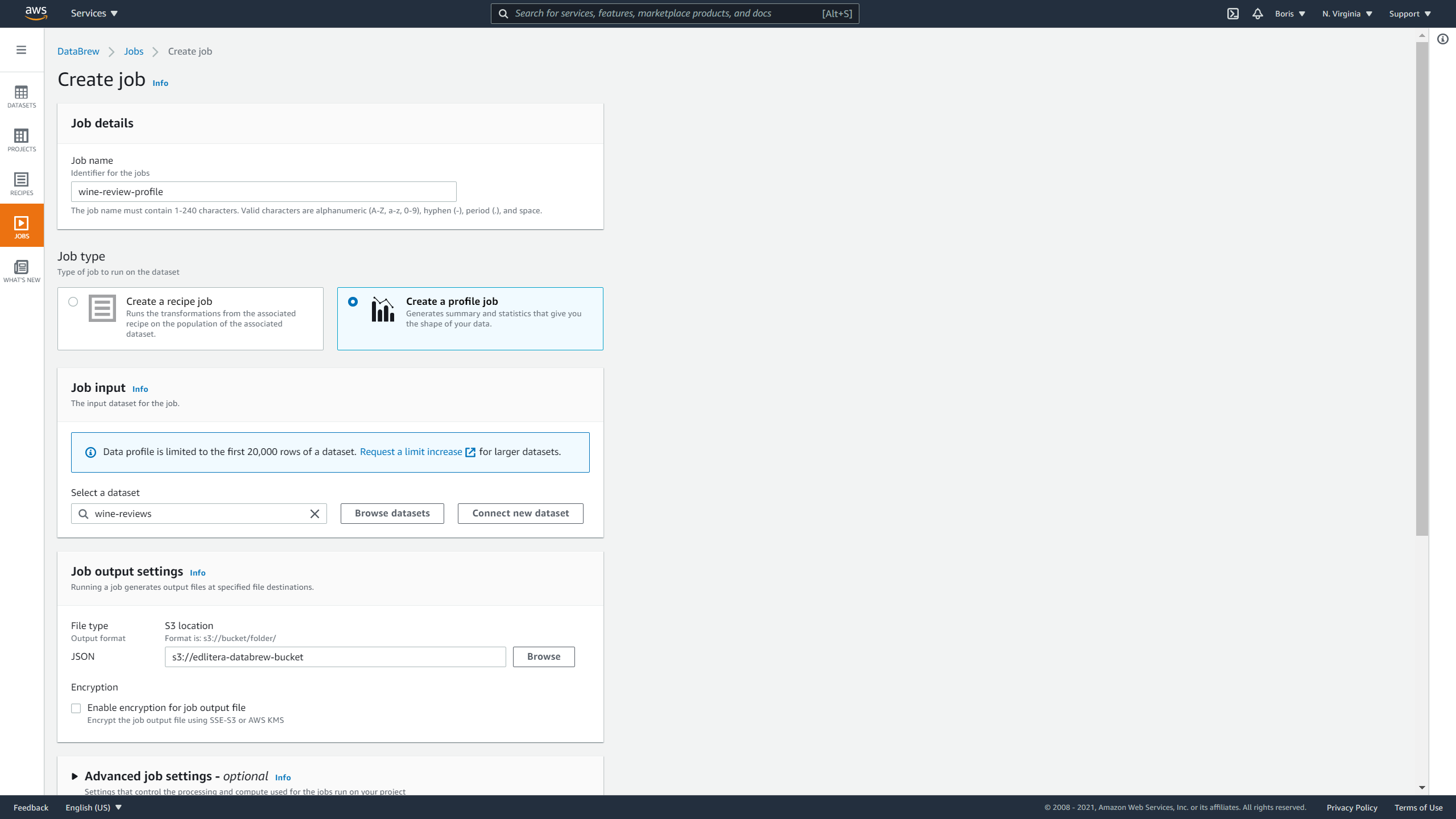
Let's call it job wine-review-profile. You will select that you want to create a profile job and select your dataset.
For output, you will select the bucket you created earlier:
Image Source: Screenshot of AWS DataBrew, Edlitera
To finish, you need to define a role.
Since you don't already have a role that you can select, you can create a new role and let's name it edlitera-profiling-job:
Image Source: Screenshot of AWS DataBrew, Edlitera
After defining everything, you just need to click on Create and run job and DataBrew will start profiling your dataset:
Image Source: Screenshot of AWS DataBrew, Edlitera
Once the job is finished, you can click on View profile which is situated in the upper right corner.
A dataset profile contains the next sections:
- Dataset preview
- Data profile overview
- Column statistics
- Data lineage
The Dataset preview section displays the dataset alongside information such as dataset name, data size, where your data is stored, etc.
Image Source: Screenshot of AWS DataBrew, Edlitera
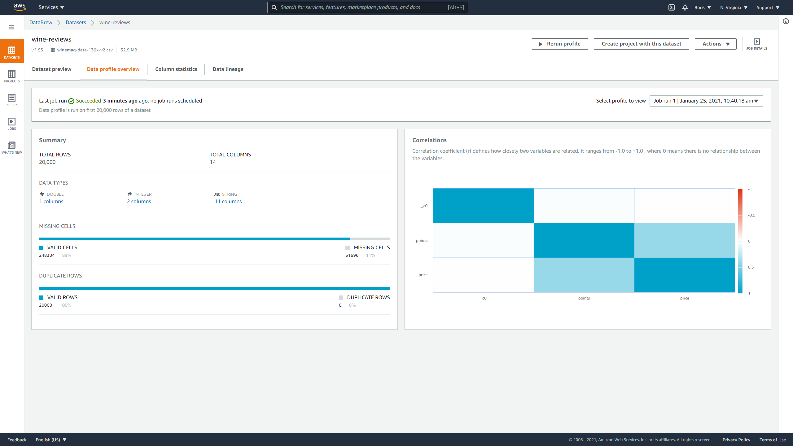
Data profile displays information about:
- Number of rows
- Number of columns
- Data types of columns
- Missing data
- Duplicate data
- Correlation matrix
Image Source: Screenshot of AWS DataBrew, Edlitera
This dataset doesn't contain duplicates, but it is missing some data.
Since the correlation matrix shows only three values and you have fourteen columns in total, you can conclude that you have a lot of columns with categorical data, which is also confirmed by the data types section.
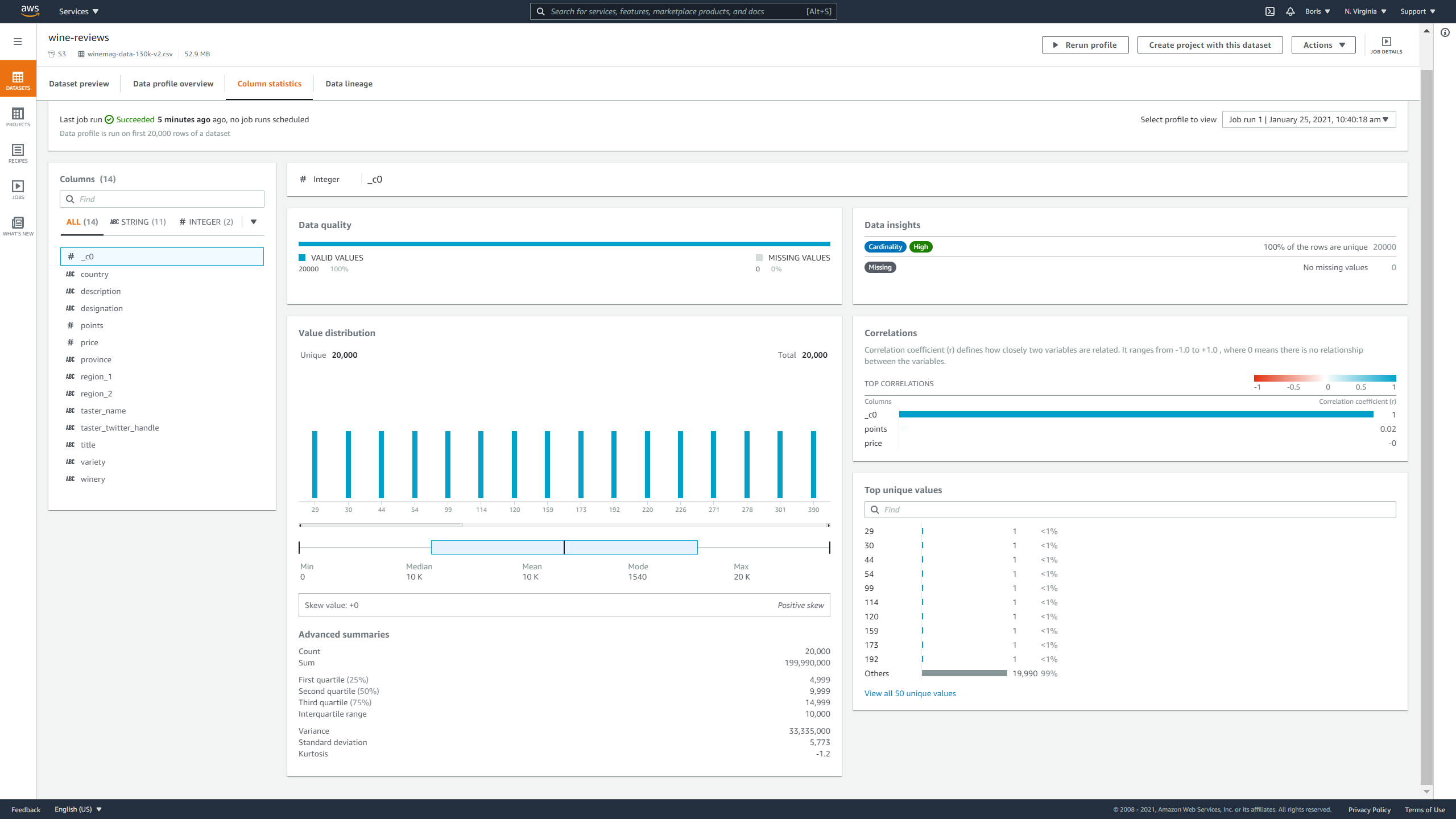
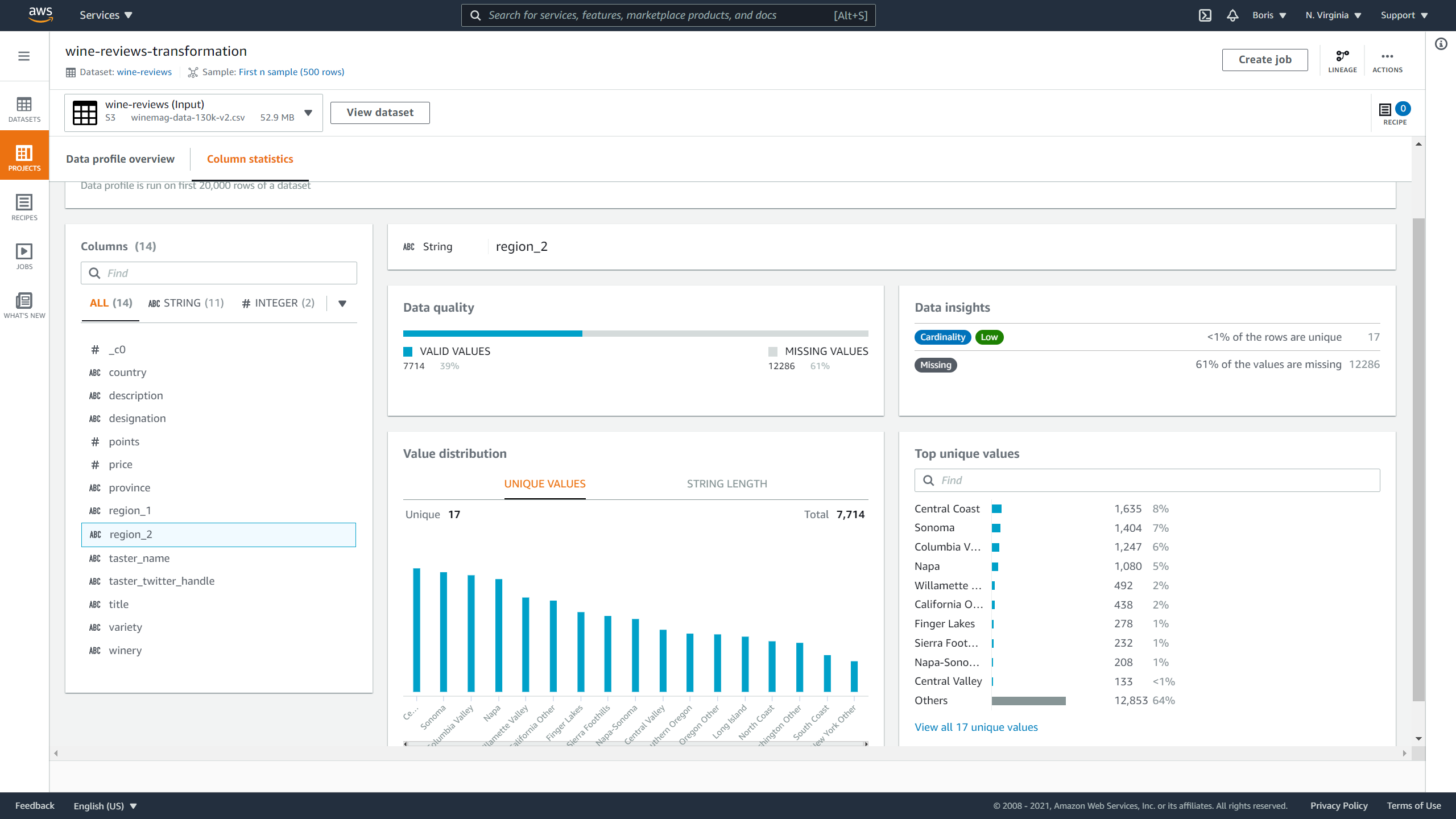
Clicking on column statistics displays the following information:
- Column data type
- Percentage of missing data in column
- Cardinality
- Value distribution graph
- Skewness factor
- Kurtosis
- Top ten most frequent unique values
- The correlation coefficient between columns
Image Source: Screenshot of AWS DataBrew, Edlitera
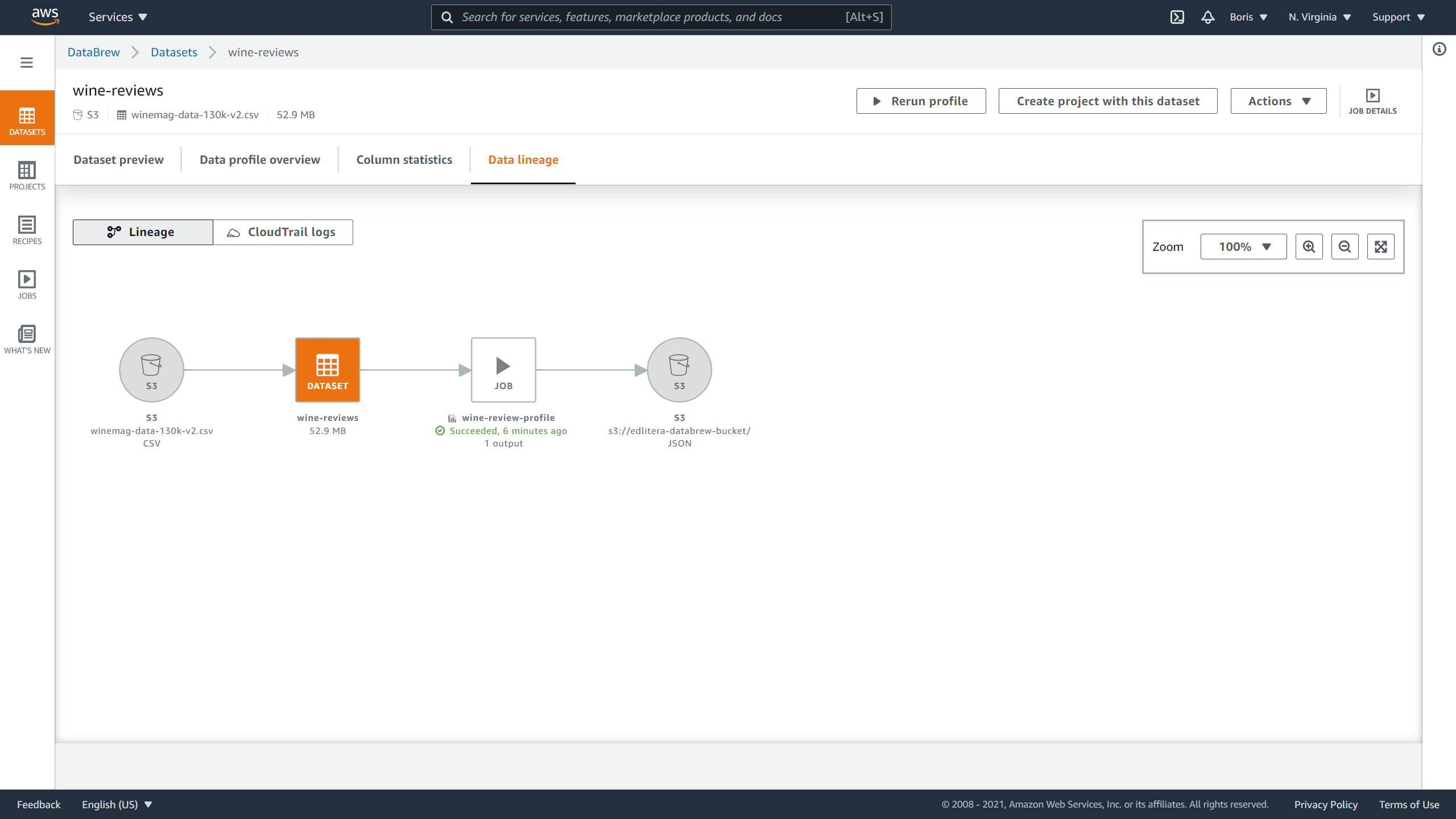
Finally, opening the Data lineage tab gives you a visual representation of the lineage of your data:
Image Source: Screenshot of AWS DataBrew, Edlitera
How to Transform Your Data
As mentioned before, this is probably the most important function of DataBrew. Transforming a dataset follows a transformation recipe, a sequence of transformations defined in a format that can be easily reused.
To demonstrate some of the functionalities that DataBrew offers, let's create a DataBrew project and define a DataBrew transformation recipe.
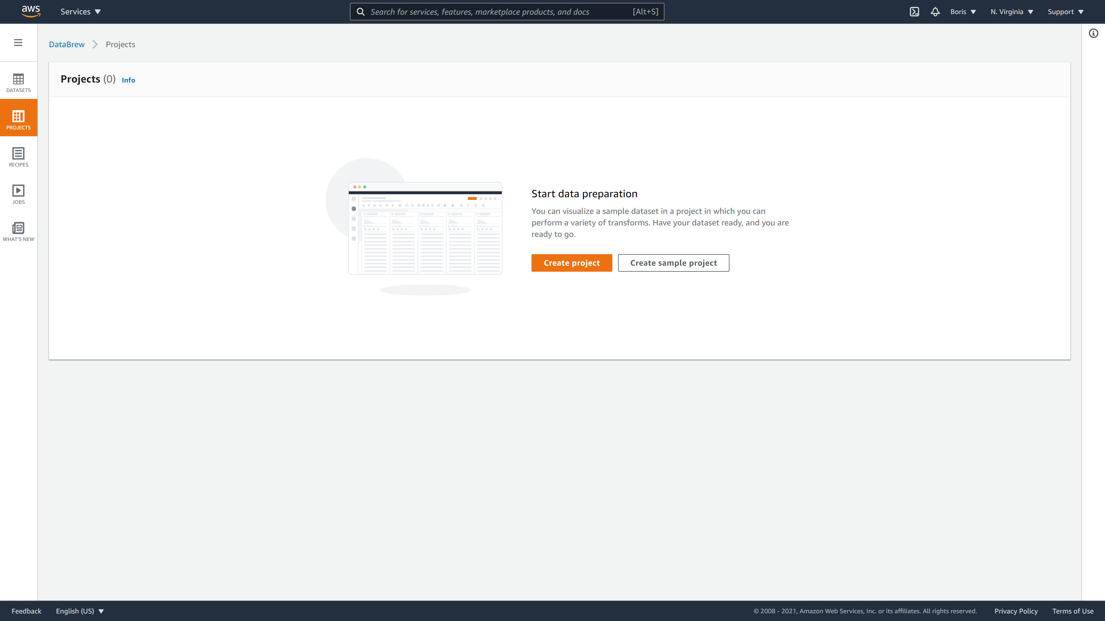
To do that, you need to click on Create project inside the Projects tab:
Image Source: Screenshot of AWS DataBrew, Edlitera
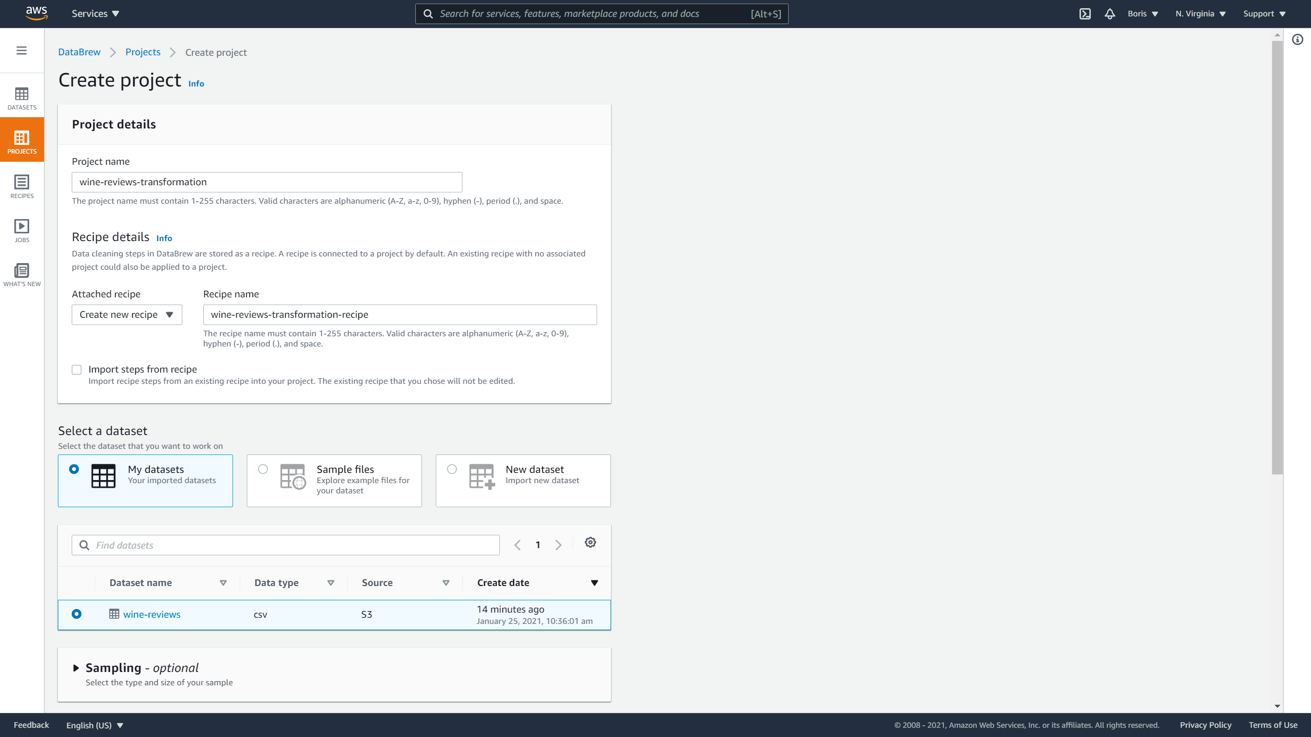
To create a project, you need to define values for the following variables:
- Project name
- Recipe name
- Dataset
- Permissions
- Sampling and tags (optional)
Let's name your project wine-reviews-transformation, and your new recipe wine-reviews-transformation-recipe.
Afterward, you are going to select that you want to work with wine-reviews dataset:
Image Source: Screenshot of AWS DataBrew, Edlitera
For Sampling, leave the value at default, which means you will take a look at a sample of 500 rows, which is enough to demonstrate how recipes are made.
To finish defining the process, select the same role that you used earlier: the AWSGlueDataBrewServiceRole-wine-reviews role:
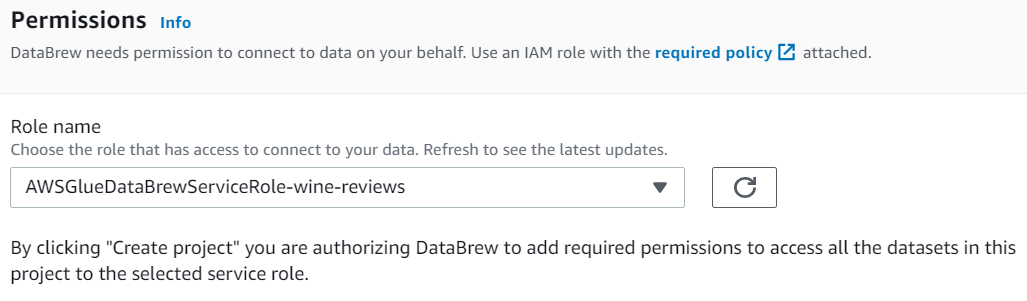
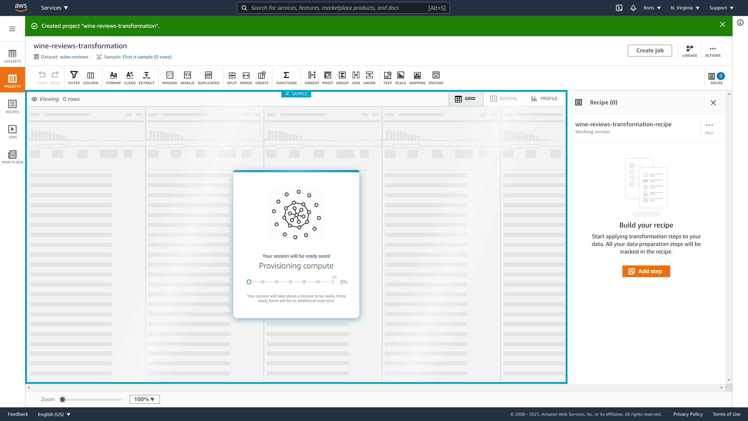
DataBrew will then start preparing a session, which takes a little bit of time:
Image Source: Screenshot of AWS DataBrew, Edlitera
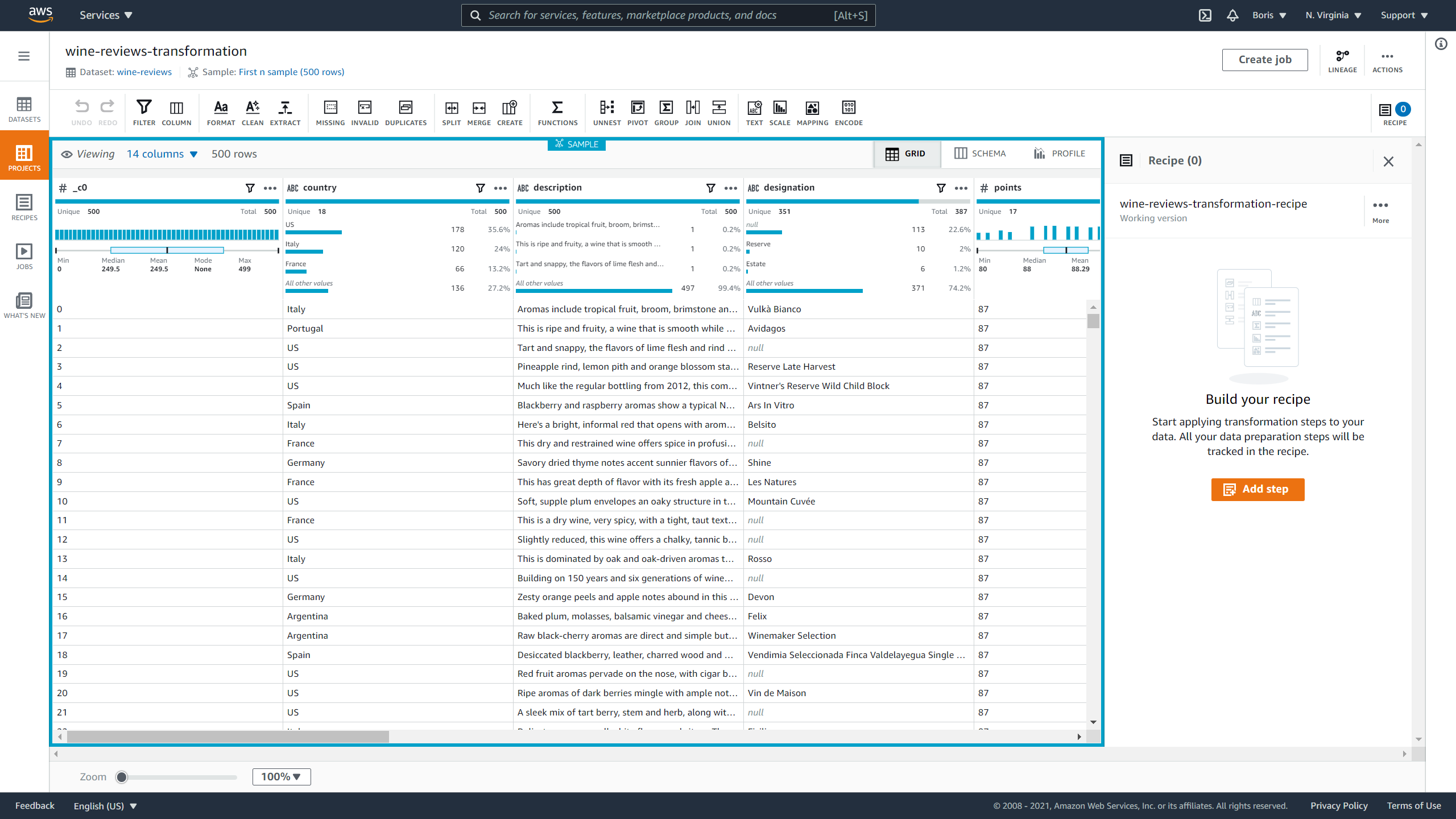
You can display your dataset as a grid or a schema.
For this demonstration, I will display it as a grid:
Image Source: Screenshot of AWS DataBrew, Edlitera
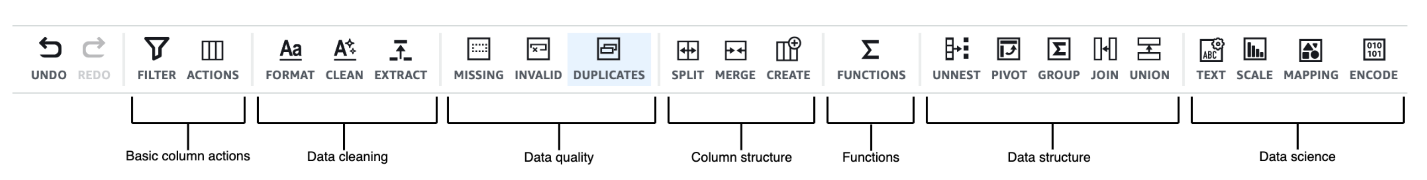
Now it is time to start building your recipe. When you click on Add step you can select a transformation that you want to apply to your dataset. The different transformations you can perform are visible in the toolbar above your dataset.
They serve many different purposes:
Image Source: Screenshot of AWS DataBrew, Edlitera
Let's start transforming your data.
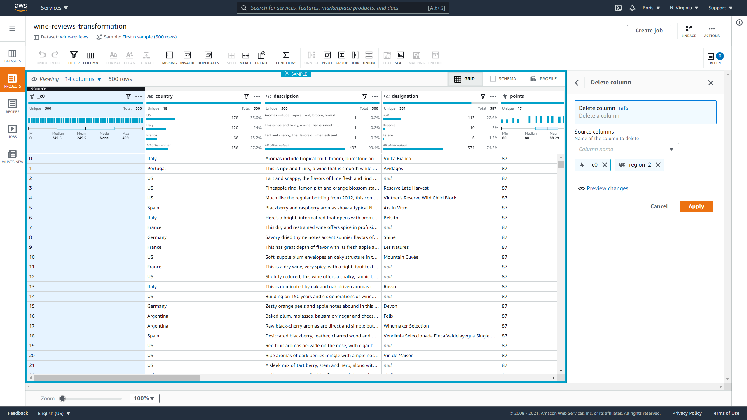
First, let's remove the _c0 column because it is a copy of the index. Next, you can see if there are any columns you can immediately discard based on how much data they are missing.
If you go back to the profile and look at each column independently, notice that the region_2 column is missing over 60% of its total data.
I will remove it because it is missing too much data:
Image Source: Screenshot of AWS DataBrew, Edlitera
To remove columns, click on Column actions and then Delete.
To finish the process, just select the columns you want to remove and click Apply.
Image Source: Screenshot of AWS DataBrew, Edlitera
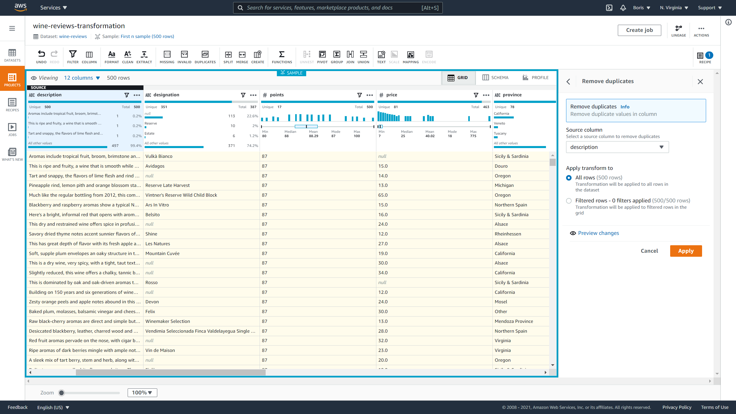
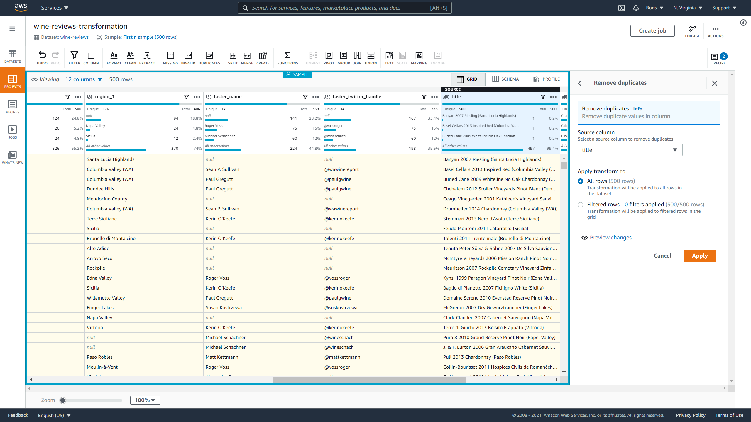
Now let's deal with duplicate values.
The current dataset doesn't have duplicates, but since you'll want to make this recipe reusable, I am going to include this step. Let's look for duplicate rows in the description and title columns. Wines can be from the same country or cost the same, but no two wines can have the same name or have the same description.
To deal with duplicates, click on Duplicate values and then click Remove duplicate values in columns. Then you just select the column that can potentially have duplicates and click Apply:
Image Source: Screenshot of AWS DataBrew, Edlitera
Image Source: Screenshot of AWS DataBrew, Edlitera
Your next step will be getting rid of missing values. You will fill in missing values with the average value if the column is a numerical one, or with the most frequent value if it is a categorical one
Let's start with the price column. That column is a numerical one.
To impute missing values, click on Missing values and then Fill or impute missing values. Then you select Numeric aggregate, select Average and click on Apply:
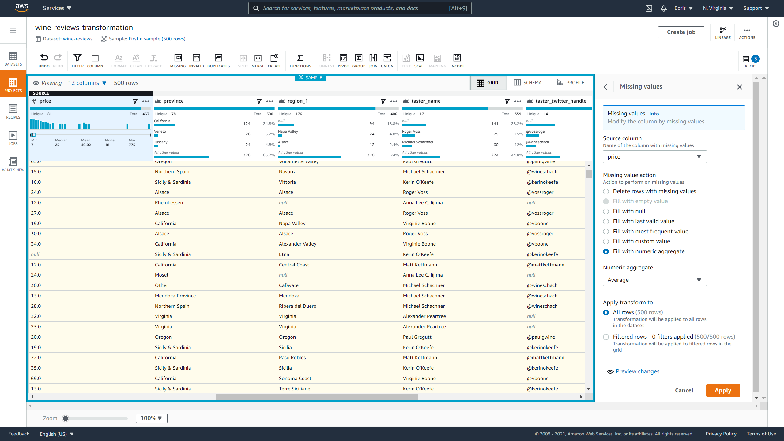
To impute a categorical column, click on Missing values and then on Fill or impute missing values, followed by Fill with most frequent value.
Apply this procedure to the Designation, region_1, taster_name, and taster_twitter_handle.
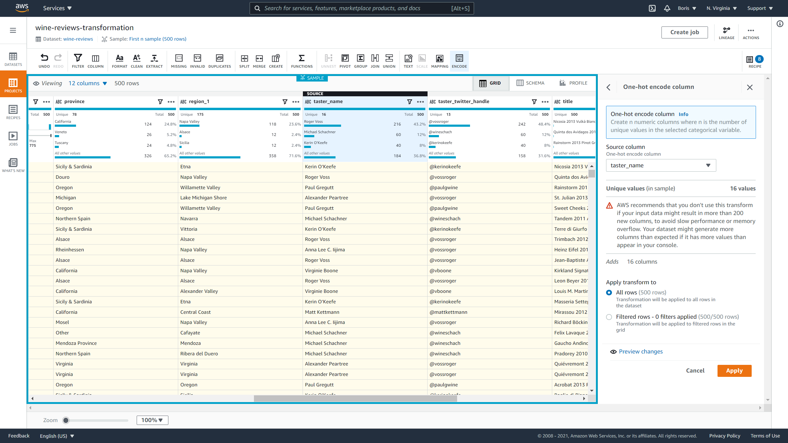
To finish, let's demonstrate how to encode categorical data. To avoid making this article too long, I won't deal with all columns and will instead demonstrate how to one-hot encode the taster_name and taster_twitter_handle columns. The number of unique values inside other columns is too big for one-hot encoding.
To one-hot encode data, you need to click on Encode and then on One-hot encode column. Select taster_name and click on Apply.
Image Source: Screenshot of AWS DataBrew, Edlitera
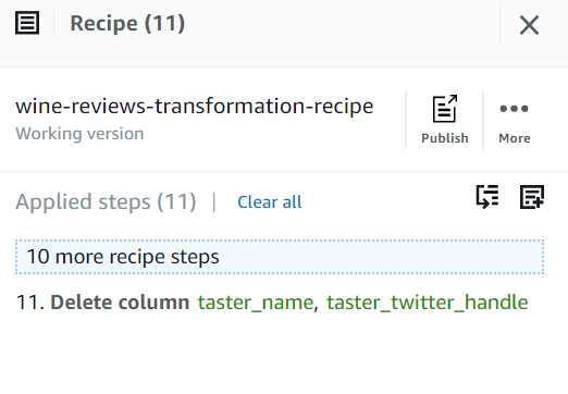
However, DataBrew won't automatically remove the original column. You'll need to do that manually in a way similar to how you discarded _c0 and region_2. To one-hot encode taster_twitter_handle you just repeat the procedure. Once these tasks have been finished, you can remove the original taster_name and taster_twitter_handle columns.
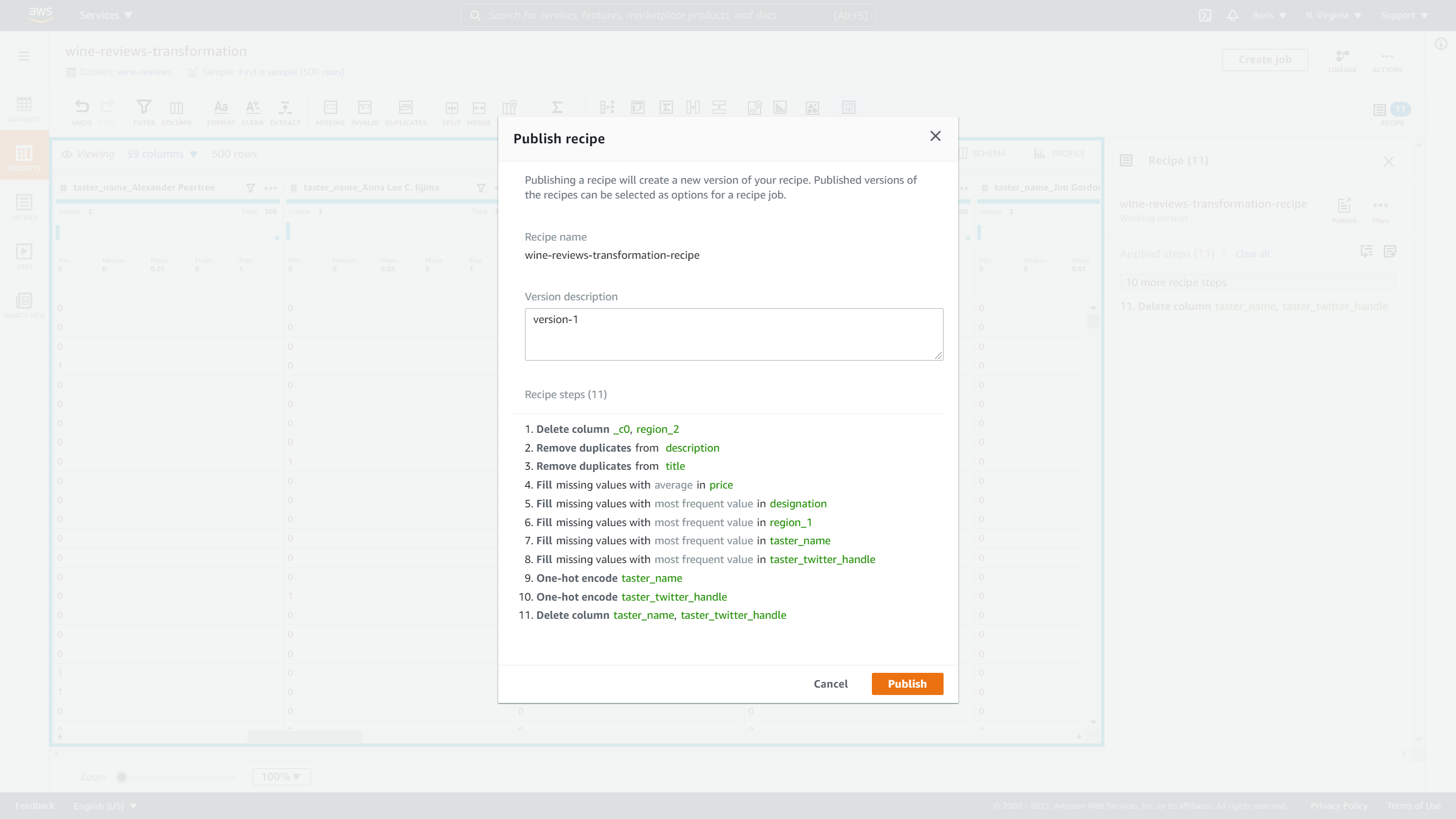
After you've finished your transformation recipe, you can publish it by clicking on Publish.
Image Source: Screenshot of AWS DataBrew, Edlitera
When publishing the recipe, under Version description you can put version-1 and click on Publish.
Image Source: Screenshot of AWS DataBrew, Edlitera
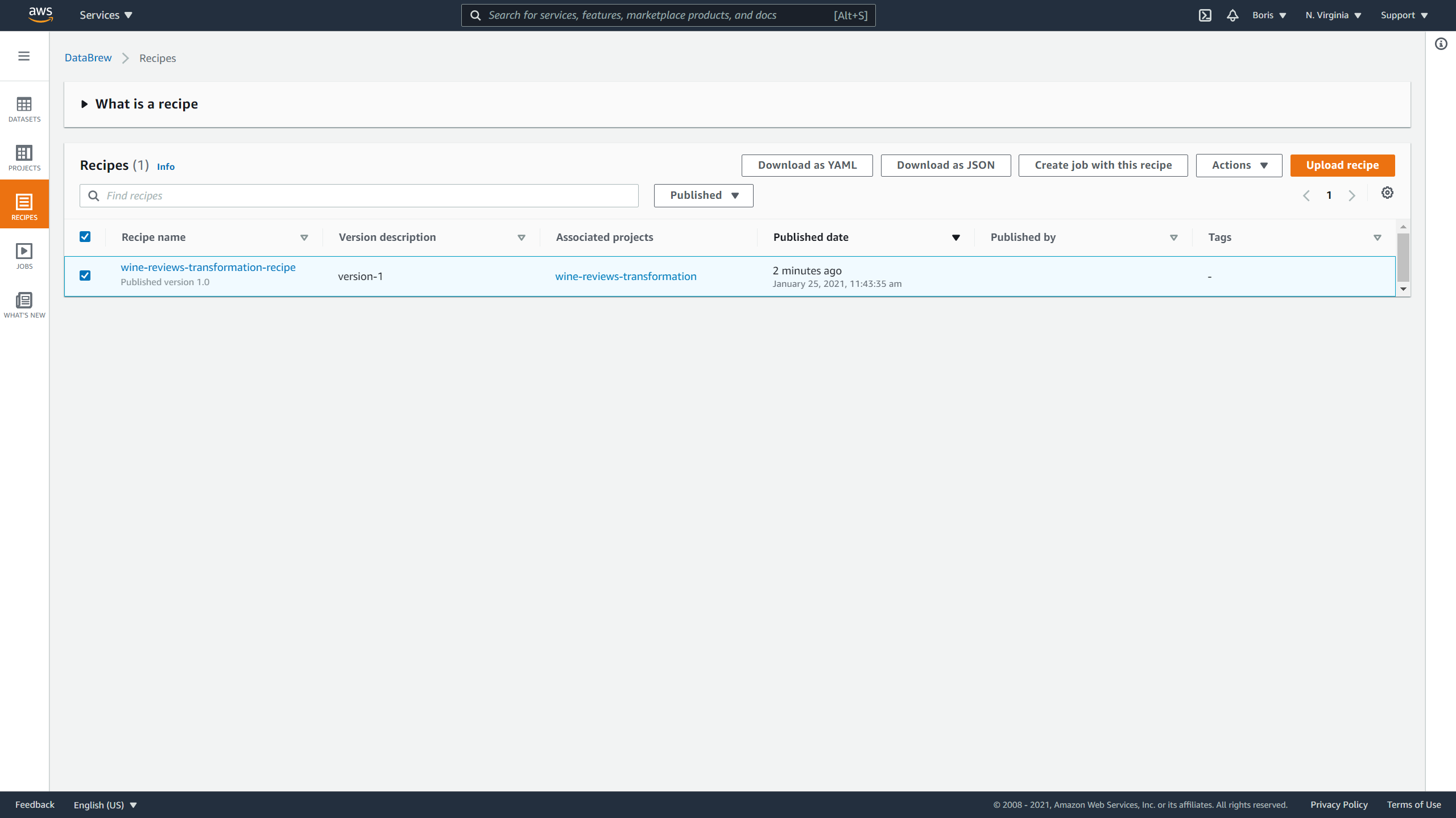
If you click on the Recipes tab now, you will see that the recipe has been successfully published.
It will also allow you to do the following actions with that recipe:
- Download it as a YAML
- Download it as JSON
- Create a job using this recipe
- Upload recipe
Image Source: Screenshot of AWS DataBrew, Edlitera
Even before DataBrew was introduced, AWS Glue was very popular. AWS is currently the most popular cloud platform, so this shouldn't come as a surprise. Even though it doesn't integrate that well with tools that are not part of AWS, most Glue users already used other AWS services so that was never a problem. The inclusion of DataBrew will most likely make Glue even more popular. With its simplicity and zero code interface, it is the perfect tool for creating an environment where a multitude of different teams from different technical backgrounds can collaborate.
However, its simplicity can also be considered its biggest flaw. Some users simply need more freedom and flexibility than DataBrew offers. Very advanced users that heavily invest in complex machine learning and deep learning methods will probably feel somewhat limited. Even if it has over 250 built-in transformations, sometimes a data scientist needs to modify a particular transformation to specifically target an issue with a model. This kind of precision is unfortunately not available without some coding, and as such is impossible to implement in a tool like DataBrew.
All in all, Glue is an excellent service even without DataBrew. DataBrew is just an addition that is aimed at a particular audience: anyone with little-to-no coding knowledge. For most people, DataBrew will be enough because it offers a lot of built-in functionality. The fact that more advanced users might decide to use a tool such as SageMaker DataWrangler doesn't invalidate DataBrew as a tool. DataBrew's limitations are not incidental and show how well its creators knew exactly what their target audience wants from such a tool. Therefore, it is important to keep in mind that DataBrew was designed to provide a lot of functionality to beginner programmers.
- Read next in series: The Ultimate Guide to Amazon SageMaker > >

