


Table of Contents
This article explores how to use pivot tables in Pandas, a key tool for summarizing large sets of data. Pivot tables help in organizing and understanding data by highlighting trends and patterns. We'll show you the basics of creating pivot tables in Pandas. This process is similar to how they work in spreadsheet programs like Excel. This is just the beginning, as we plan to cover the groupby method in Pandas in our upcoming articles for more advanced data analysis.
Article continues below
Want to learn more? Check out some of our courses:
What are Pivot Tables
Pivot tables are, in general, important tools used to summarize and analyze large quantities of data. They allow us to easily rearrange, sort, and filter data. This is done in a way where it becomes easier to identify patterns and trends that might not be immediately obvious. In Python, pivot tables are used primarily for data analysis. Even though we create and manipulate them using code, in concept the pivot tables from Python are highly similar to pivot tables in spreadsheet software, such as Excel.
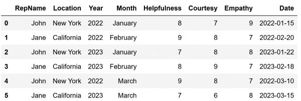
Let's demonstrate how we can summarize data using pivot tables in Pandas. For starters, I am going to create a DataFrame that can be used as an example:
import pandas as pd

# Create some example data
data= {
    "RepName": ["John", "Jane", "John", "Jane", "John", "Jane"],
    "Location": ["New York", "California", "New York", "California", "New York", "California"],
    "Year": [2022, 2022, 2023, 2023, 2022, 2023],
    "Month": ["January", "February", "January", "February", "March", "March"],
    "Helpfulness": [8, 9, 7, 8, 9, 7],
    "Courtesy": [7, 8, 8, 9, 8, 6],
    "Empathy": [9, 7, 8, 7, 7, 8],
    "Date": pd.to_datetime(["2022-01-15", "2022-02-20", "2023-01-22", "2023-02-18", "2022-03-10", "2023-03-15"])
}


# Create the DataFrame
df = pd.DataFrame(data)
The code above will create the following DataFrame and store it in the df variable:
How to Create Simple Pivot Tables
To create a pivot table using Pandas we use the pivot_table method, which we apply directly to the DataFrame that contains our data. When using the pivot_table method we need to define values for a few arguments:
• index
• columns
• values
• aggfunc
There are also some other arguments for which we can define values. However, we will focus more on that later, as we get to creating complex pivot tables.
The index argument indicates the keys by which to group the data on the pivot table index. It fundamentally defines what are we going to use as row labels in our pivot table.
The columns argument indicates the keys by which to group the data on the pivot table column. Using this argument we define what we want to use as column labels in the pivot table.
The values argument indicates which columns we want to aggregate. It can be one column or multiple columns and is an optional argument. In other words, if no value is provided for this argument, the pivot table will automatically use all numeric columns during its creation.
Finally, the aggfunc argument indicates the aggregation functions we want to use i.e. the mathematical function (such as mean, sum, etc.) to be used to summarize our data.
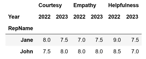
Let's create a simple pivot table, that will show the average ratings for 'Helpfulness', 'Courtesy', and 'Empathy' for each representative throughout the years.
# Creating a basic pivot table
pivot_table_basic = df.pivot_table(
    index='RepName',
    columns='Year',
    values=['Helpfulness', 'Courtesy', 'Empathy'],
    aggfunc='mean'
)
The code above will create the following pivot table and store it inside the pivot_table_basic variable:
To get the pivot table you see above, Pandas is going to perform a few operations in the background.
It first selects the relevant data from the DataFrame based on the specific parameters that we entered.
Then it groups the data by RepName for rows and by Year for columns. This is done because those are the two values we entered for the index and columns arguments. To group the data Pandas creates a hierarchical index for the rows and columns.
Afterward, it applies the aggregation function we defined via the aggfunc argument to our grouped data. This process involves iterating over each group, calculating the result of applying the function (in this case we are calculating the mean), and storing the result.
Lastly, the data is reshaped into the pivot table format before being returned to us. There is one step that happens in between the reshaping and the pivot table being returned to us and that is handling missing values. If we run into a situation where we have combinations of our row index labels and column index labels that don't exist in the original data (in this case if there are combinations of RepName and Year that don’t exist in the original data), Pandas will fill these cells with NaN values.
- Intro to Pandas: How to Create Pivot Tables in Pandas
- Intro to Pandas: How to Analyze Pandas DataFrames
How to Create Complex Pivot Tables
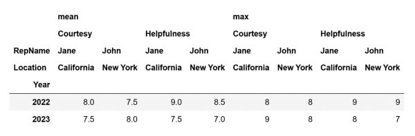
We can also create more complex pivot tables, aside from creating simple pivot tables. For instance, in the previous DataFrame we entered a single value for most of our arguments. However, we can also enter multiple values. For instance, let's create a pivot table that displays both average and peak ratings of helpfulness and courtesy for each representative across different locations, analyzed year by year.
# Create a complex pivot table
pivot_table_complex = df.pivot_table(
    index='Year',
    columns=['RepName','Location'],
    values=['Helpfulness', 'Courtesy'],
    aggfunc=['mean', 'max']
)
The code above will create the following pivot table and store it inside the pivot_table_complex variable:
As can be seen, the pivot table above is considerably more complex than the one we initially created. However, do not fear such a process because creating such a pivot table and reading it is not that hard. Let's break it down.
index
• the pivot table is indexed by Year, meaning each row corresponds to a different year
• this setup allows for an annual comparison and shows how the ratings change from year to year
columns
• there are two levels of columns, combining RepName and Location
• the first level is the name of the representative, and the second level is their location
• this arrangement enables a detailed comparison of representatives' performances across different locations
values
• the pivot table focuses on two metrics that we want to analyze: Helpfulness and Courtesy
• by focusing on these two metrics we get a good idea of how helpful and courteous the representatives are in their customer interactions
aggfunc
• two different statistical measures are used
• the 'mean' gives an average rating, showing the general level of performance, while the 'max' indicates the peak performance for each category
Therefore, even though the pivot table might seem especially complex at first, if you understand what each of the different arguments in the pivot_table method represents, constructing and reading the table ends up a significantly simple task.
What are the Additional Arguments
As mentioned previously in the article, aside from the main four arguments, others can also play an important role in certain situations. Those are:
• fill_value - value to replace missing values with
• margins - if set to True, add all row/column combinations with subtotals at the bottom/right
• dropna - if set to True, rows with a NaN value in any column will be omitted before computing margins
• margins_name - the name of the row/column that will contain the totals when the margins argument value is set to True
• sort - specifies if the result should be sorted
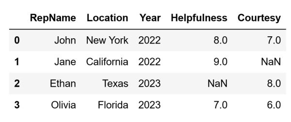
To demonstrate how we can use these arguments the DataFrame needs to be more complex. Its current version is not complex enough to justify the usage of these additional arguments. Let's create a new DataFrame, similar to the one we originally used. This new one is going to have values that are more varied and will also contain some missing values:
# Create a new DataFrame
sample_data = {
    "RepName": ["John", "Jane", "Ethan", "Olivia"],
    "Location": ["New York", "California", "Texas", "Florida"],
    "Year": [2022, 2022, 2023, 2023],
    "Helpfulness": [8, 9, None, 7],
    "Courtesy": [7, None, 8, 6]
}
sample_df = pd.DataFrame(sample_data)
The code above is going to create the following DataFrame and store it inside the sample_df variable:
Now that we have a new DataFrame to work with, let's create a pivot table. That will provide a summarized view of the Helpfulness and Courtesy ratings by a representative (RepName) for each year, along with totals and handling of missing values.
# Pivot table with additional parameters
pivot_table_example = sample_df.pivot_table(
    index='Year',
    columns='RepName',
    values=['Helpfulness', 'Courtesy'],
    aggfunc='mean',
    fill_value=0,         # Replaces missing values with 0
    margins=True,         # Adds subtotals at the bottom/right
    dropna=False,         # Keep data even if you run into NaN values
    margins_name='Total', # Name for the totals row/column
    sort=True             # Sorts the result
)
The code above is going to create the following DataFrame and store it inside the pivot_table_example variable:
Out of the aforementioned, the most important one is likely the margins argument. The reason for this is that adding subtotals to your pivot table is something that you will do quite often. These subtotals are additional rows and/or columns that provide aggregated data across different levels of your grouping variables. We have three types of subtotals:
• row subtotals
• column subtotals
• grand totals
If your pivot table is grouped by one or more row indices, a row subtotal will provide aggregated data across all these groups. For example, if your rows are indexed by 'Year', the row subtotal will provide the aggregated data for all years.
Similarly, if your pivot table has one or more column indices, a column subtotal will aggregate data across all these columns. For instance, if your columns represent different representatives, the column subtotal will provide the aggregated data for all representatives.
Lastly, in addition to subtotals for each level of your index or columns, margins=True also adds a total. This is the overall aggregation across all rows and columns. Essentially, it provides a summary statistic (like mean, sum, etc.) for the entire dataset included in the pivot table.
The subtotals and total provide a useful high-level summary of the data. This results in making it easier to understand overall trends and comparisons across different groups. The names of these subtotal rows/columns can be customized using the margins_name argument. Setting a value for this argument gives you the chance to personalize the labels for the subtotal rows/columns in your pivot table, thus you will often prefer to do so.
- Pandas vs Excel: Which Is the Best for Data Analysis?
- The Ultimate Guide to Data Processing with Python
To sum up, pivot tables in Pandas are a great way to make sense of complex data. They allow us to break down and analyze data in an organized way. This article has laid the groundwork for understanding these pivot tables, both the simple and complex ones. We will build on this with more tools like the groupby method in future discussions. These tools are invaluable for anyone looking to delve deeper into data analysis.

![[Future of Work Ep. 2 P3] Future of Learning and Development with Dan Mackey: Learning Data](https://res.cloudinary.com/edlitera/image/upload/ar_16:9,c_fill,f_auto,q_auto,w_100/z4omald0x6c7isoqhgf2w7skd3x0?_a=BACADKBn)